Least Squares Sinusoidal Parameter Estimation

There are many ways to define ``optimal'' in signal modeling. Perhaps the most elementary case is least squares estimation. Every estimator tries to measure one or more parameters of some underlying signal model. In the case of sinusoidal parameter estimation, the simplest model consists of a single complex sinusoidal component in additive white noise:

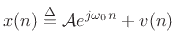$$x(n) \isdef {\cal A}e^{j\omega_0 n} + v(n) \protect$$ (6.32)

where ${\cal A}= A e^{j\phi}$ is the complex amplitude of the sinusoid, and $v(n)$ is white noise (defined in §C.3). Given measurements of $x(n)$ , $n=0,1,2,\ldots,N-1$ , we wish to estimate the parameters $(A,\phi,\omega_0 )$ of this sinusoid. In the method of least squares, we minimize the sum of squared errors between the data and our model. That is, we minimize

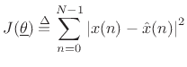$$J(\underline{\theta}) \isdef \sum_{n=0}^{N-1}\left\vert x(n)-{\hat x}(n)\right\vert^2 \protect$$ (6.33)

with respect to the parameter vector

$$\underline{\theta}\isdef \left[\begin{array}{c} A \\ [2pt] \phi \\ [2pt] \omega_0 \end{array}\right],$$ (6.34)

where ${\hat x}(n)$ denotes our signal model:

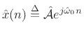$${\hat x}(n)\isdef \hat{{\cal A}}e^{j\hat{\omega}_0n}$$ (6.35)

Note that the error signal $x(n)-\hat{{\cal A}}e^{j\hat{\omega}_0n}$ is linear in $\hat{{\cal A}}$ but nonlinear in the parameter $\hat{\omega}_0$ . More significantly, $J(\underline{\theta})$ is non-convex with respect to variations in $\hat{\omega}_0$ . Non-convexity can make an optimization based on gradient descent very difficult, while convex optimization problems can generally be solved quite efficiently [22,86].