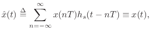
We review briefly the ``analog interpretation'' of sampling rate conversion
[97] on which the present method is based. Suppose we have
samples ![]() of a continuous absolutely integrable signal
of a continuous absolutely integrable signal ![]() ,
where
,
where ![]() is time in seconds (real),
is time in seconds (real), ![]() ranges over the integers, and
ranges over the integers, and
![]() is the sampling period. We assume
is the sampling period. We assume ![]() is bandlimited to
is bandlimited to
![]() , where
, where ![]() is the sampling rate. If
is the sampling rate. If ![]() denotes the Fourier transform of
denotes the Fourier transform of ![]() , i.e.,
, i.e.,
![]() , then we assume
, then we assume
![]() for
for
![]() . Consequently, Shannon's sampling
theorem gives us that
. Consequently, Shannon's sampling
theorem gives us that ![]() can be uniquely reconstructed from the
samples
can be uniquely reconstructed from the
samples ![]() via
via
where
To resample
When the new sampling rate
![]() is less than the original rate
is less than the original rate ![]() ,
the lowpass cutoff must be placed below half the new lower sampling rate.
Thus, in the case of an ideal lowpass,
,
the lowpass cutoff must be placed below half the new lower sampling rate.
Thus, in the case of an ideal lowpass,
![]() sinc
sinc![]() , where the scale factor maintains unity gain
in the passband.
, where the scale factor maintains unity gain
in the passband.
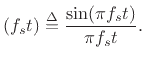
A plot of the sinc function
sinc![]() to the left and right of the origin
to the left and right of the origin ![]() is shown in Fig.4.21.
Note that peak is at amplitude
is shown in Fig.4.21.
Note that peak is at amplitude ![]() , and zero-crossings occur at all
nonzero integers. The sinc function can be seen as a hyperbolically
weighted sine function with its zero at the origin canceled out. The
name sinc function derives from its classical name as the
sine cardinal (or cardinal sine) function.
, and zero-crossings occur at all
nonzero integers. The sinc function can be seen as a hyperbolically
weighted sine function with its zero at the origin canceled out. The
name sinc function derives from its classical name as the
sine cardinal (or cardinal sine) function.
If ``![]() '' denotes the convolution operation for digital signals, then
the summation in Eq.(4.13) can be written as
'' denotes the convolution operation for digital signals, then
the summation in Eq.(4.13) can be written as
![]() .
.
Equation Eq.(4.13) can be interpreted as a superpositon of
shifted and scaled sinc functions ![]() . A sinc function instance is
translated to each signal sample and scaled by that sample, and the
instances are all added together. Note that zero-crossings of
sinc
. A sinc function instance is
translated to each signal sample and scaled by that sample, and the
instances are all added together. Note that zero-crossings of
sinc![]() occur at all integers except
occur at all integers except ![]() . That means at time
. That means at time
![]() , (i.e., on a sample instant), the only contribution to the
sum is the single sample
, (i.e., on a sample instant), the only contribution to the
sum is the single sample ![]() . All other samples contribute sinc
functions which have a zero-crossing at time
. All other samples contribute sinc
functions which have a zero-crossing at time ![]() . Thus, the
interpolation goes precisely through the existing samples, as it
should.
. Thus, the
interpolation goes precisely through the existing samples, as it
should.
A plot indicating how sinc functions sum together to reconstruct
bandlimited signals is shown in Fig.4.22. The figure shows a
superposition of five sinc functions, each at unit amplitude, and
displaced by one-sample intervals. These sinc functions would be used
to reconstruct the bandlimited interpolation of the discrete-time
signal
![]() . Note that at each sampling
instant
. Note that at each sampling
instant ![]() , the solid line passes exactly through the tip of the
sinc function for that sample; this is just a restatement of the fact
that the interpolation passes through the existing samples. Since the
nonzero samples of the digital signal are all
, the solid line passes exactly through the tip of the
sinc function for that sample; this is just a restatement of the fact
that the interpolation passes through the existing samples. Since the
nonzero samples of the digital signal are all ![]() , we might expect the
interpolated signal to be very close to
, we might expect the
interpolated signal to be very close to ![]() over the nonzero interval;
however, this is far from being the case. The deviation from unity
between samples can be thought of as ``overshoot'' or ``ringing'' of
the lowpass filter which cuts off at half the sampling rate, or it can
be considered a ``Gibbs phenomenon'' associated with bandlimiting.
over the nonzero interval;
however, this is far from being the case. The deviation from unity
between samples can be thought of as ``overshoot'' or ``ringing'' of
the lowpass filter which cuts off at half the sampling rate, or it can
be considered a ``Gibbs phenomenon'' associated with bandlimiting.
 |
A second interpretation of Eq.(4.13) is as follows: to obtain the
interpolation at time ![]() , shift the signal samples under one sinc
function so that time
, shift the signal samples under one sinc
function so that time ![]() in the signal is translated under the peak of the
sinc function, then create the output as a linear combination of signal
samples where the coefficient of each signal sample is given by the value
of the sinc function at the location of each sample. That this
interpretation is equivalent to the first can be seen as a result of the
fact that convolution is commutative; in the first interpretation, all
signal samples are used to form a linear combination of shifted sinc
functions, while in the second interpretation, samples from one sinc
function are used to form a linear combination of samples of the shifted
input signal. The practical bandlimited interpolation algorithm presented
below is based on the second interpretation.
in the signal is translated under the peak of the
sinc function, then create the output as a linear combination of signal
samples where the coefficient of each signal sample is given by the value
of the sinc function at the location of each sample. That this
interpretation is equivalent to the first can be seen as a result of the
fact that convolution is commutative; in the first interpretation, all
signal samples are used to form a linear combination of shifted sinc
functions, while in the second interpretation, samples from one sinc
function are used to form a linear combination of samples of the shifted
input signal. The practical bandlimited interpolation algorithm presented
below is based on the second interpretation.

![\includegraphics[width=3in]{eps/Sinc}](img1150.png)