Empirical Analysis

We have modified the algorithm for the rectilinear mesh in such a way that Schroeder's diffuser is implemented on one of its boundaries, and compared them by visualizing the meshes at different time frames. Figure 5 shows wave propagation on the rectilinear mesh with rigid, flat boundaries which yield specular reflections when given an initial excitation at the center.

Figure 5: Wave propagation on the mesh with flat surfaces at time frames $n=1, 20, 40, 60, 100,$ respectively.

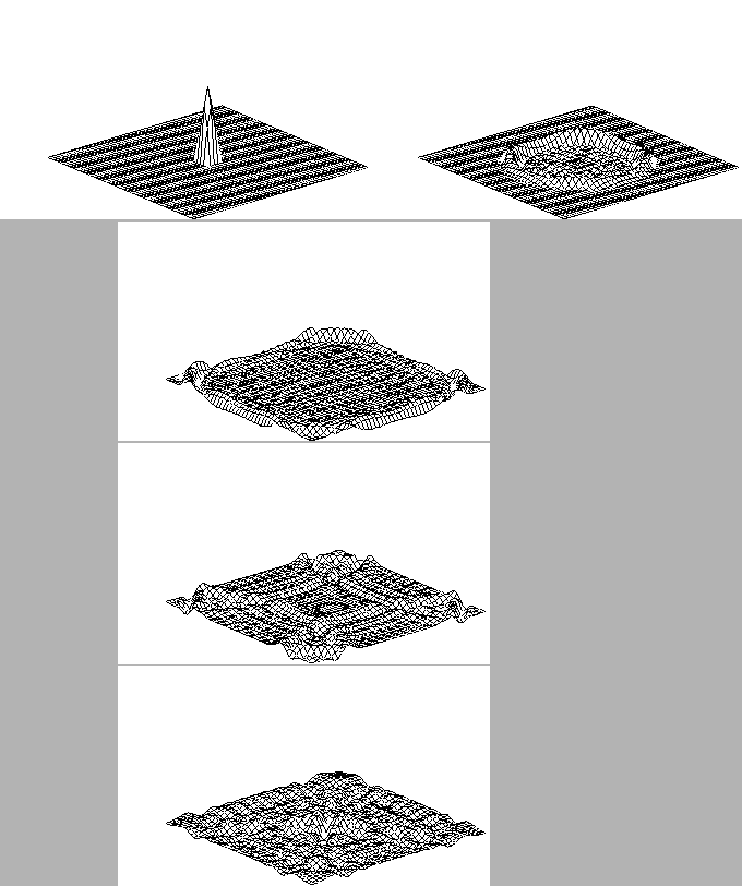
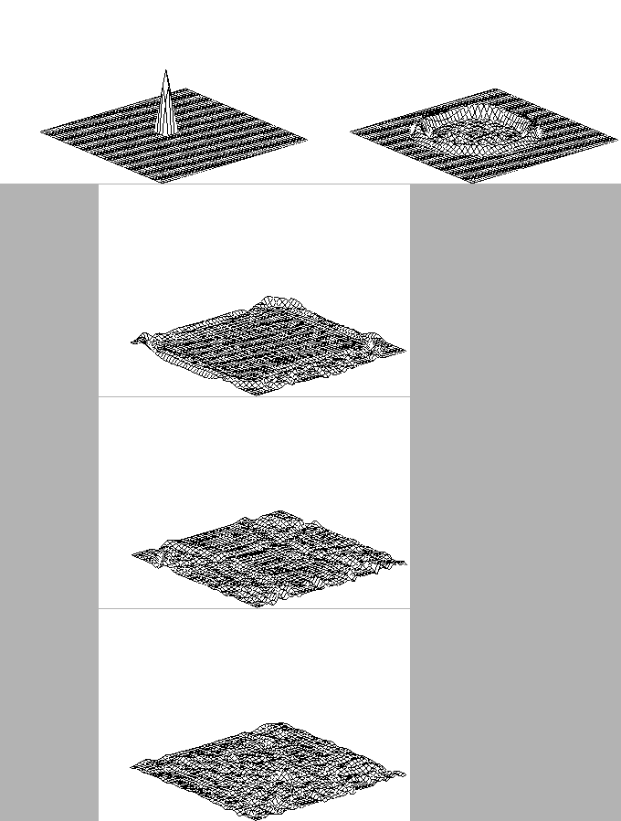
The figure shows that specular reflections occur at the boundaries. We can clearly see the symmetry in the wave propagation pattern, and the energy is concentrated at some regions in the mesh after some time has passed. On the other hand, the mesh with one of its boundaries being replaced with Schroeder's diffuser reveals very different reflection characteristics as shown in Figure 6. The wave propagates in the same pattern at the beginning as in the plain mesh, but it starts to diffuse in the third plot as it approaches a boundary with Schroeder's diffuser. This diffusion from the the uneven boundary disturbs the symmetric wave propagation pattern seen in the plain mesh, and in the last plot, we can see the energy is evenly distributed all over the mesh after a very short period of 4.5 milliseconds.

Figure 6: Wave propagation on the mesh with Schroeder's diffuser when N = 17 (diffusing surface at bottom-right side).

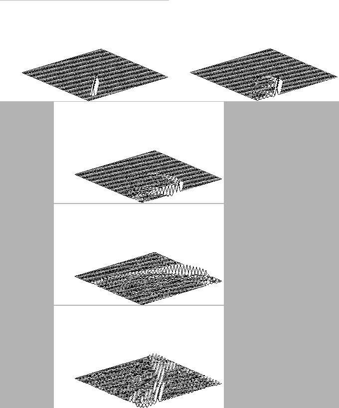
The comparison between the plain mesh with specular boundaries and the mesh with a diffusing boundary becomes more obvious if we use an incident plane wave as their initial excitation. Even before looking at the animated results, we may expect that the plain mesh with flat surfaces will show a specular reflection pattern; i.e., the plane wave will reflect with equal angles of incidence and reflection as light is reflected in the mirror. Figure 7 shows this specular reflection of the plane wave when the angle of incidence is $\alpha = 45^\circ$. The plane wave is reflected with the same angle as its angle of incidence, and keeps the same specular reflection pattern, resulting in the propagation pattern similar to diamond shape, whereas the wave propagation pattern shown in Figure 8 is totally different. The plane wave is diffused as it reaches the diffusing surface in the second plot, and it starts to propagate in many directions as shown in the next plot. Finally, in the last plot, we can see the sound energy is evenly distributed on the mesh without any visible concentration on specific regions.

Figure 7: Plane wave propagation on the mesh with flat surfaces at time frames $n=1, 10, 20, 60, 200,$ respectively.

Figure 8: Plane wave propagation on the mesh with Schroeder's diffuser when N = 17 (diffusing surface at bottom-right side).

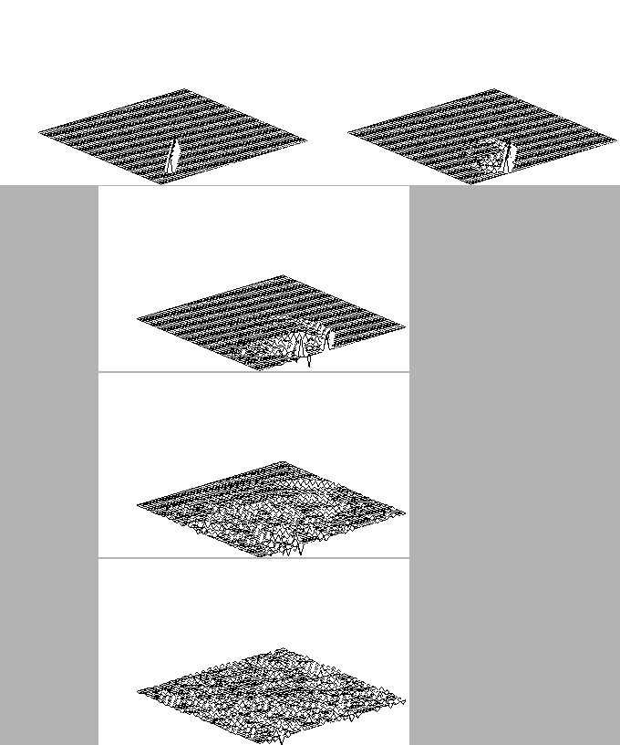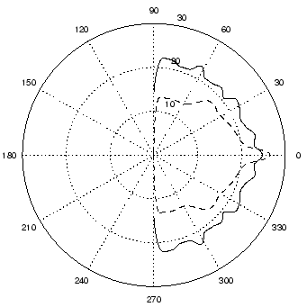
Figure 9 shows the scattering characteristics of two different meshes by using a plane wave normal to the boundary as an excitation source (i.e., incidence angle of $0^\circ$), and by picking up the output at various angles. This polar response clearly shows that the sound energy is evenly scattered at every angle at the diffusing boundary whereas only specular reflection occurs at the flat surface.

Figure 9: Scattering levels from a Schroeder's diffuser (solid) and a flat surface (dashed).

Note that sound examples and Matlab generated movies which clearly visualize wave propagation are available from the WWW URL address: http://www-ccrma.stanford.edu/~kglee/2dmesh_QRD/