Implementation of Boundary with the Wells

The 2-D digital waveguide mesh can be implemented by having bi-directional unit delay lines between adjacent junctions as shown in Figure 3.

Figure 3: The 2-D digital waveguide mesh with bi-directional unit delay lines.

picture(4674,4674)(889,-4423) (2258,-1898)(0,0)[lb] $z^{-1}$% (2858,-2963)(0,0)[lb] $z^{-1}$% (2258,-2356)(0,0)[lb] $z^{-1}$% (3308,-1313)(0,0)[lb] $z^{-1}$% (3308,-2963)(0,0)[lb] $z^{-1}$% (3908,-1913)(0,0)[lb] $z^{-1}$% (2858,-1313)(0,0)[lb] $z^{-1}$% (3908,-2363)(0,0)[lb] $z^{-1}$%

In order to simulate the boundary with the wells of different depths in a 2-D digital waveguide mesh, we need to convert the depths of the wells in Equation 4 to the number of junctions. Since the travel time of the wave in the $n$th well is given by

$$t_n = \frac{d_n}{c},$$ (10)

where $d_n$ is the depth of the $n$th well, and $c$ is the speed of the sound, we can calculate the travel time in samples for the traveling wave by multiplying Equation 10 by the sampling rate, i.e.,

$$n_n = t_nf_s = \frac{d_n}{c}f_s,$$ (11)

where $n_n$ is the travel time in samples in the $n$th well and $f_s$ is the sampling rate. Substituting $d_n$ with that in Equation 4 yields

$$n_n = \frac{\lambda_0}{2N}\frac{f_s}{c}s_n ,$$ (12)

where $s_n$ is a quadratic residue sequence with period $N$.

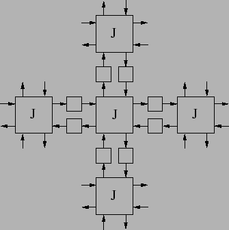
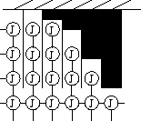
Since the wells are rigidly separated from each other in Schroeder's diffuser, we need to take this into account when implementing it in a 2-D digital waveguide mesh. This can be accomplished by disconnecting all the horizontal strings between adjacent junctions in the wells as shown in Figure 4. The disconnection of the strings between junctions means the junctions in the wells are no more considered 4-port junctions, and this changes the scattering coefficients. In fact, the junctions in the wells are now pure digital delay lines without any scattering, having reflections only at the end of the wells. The junctions are terminated at the boundaries with a reflection coefficient of 0.99.

Figure 4: The 2-D digital waveguide mesh in the vicinity of diffusing boundary. Note there are no horizontal connections between junctions in the wells.

The design wavelength $\lambda_0$ used in our simulation is 25 $cm$, and each well is one sample wide, which gives the well width of $w = cT = c/f_s \approx 1.56\:cm\:(\ll \lambda_0)$. Therefore, the $\lambda_0\gg w$ requirement in Schroeder's diffuser has been satisfied.