DISCRETISATION

In order to represent a half-hole model in a wave digital modelling context, a decomposition of the instantaneous variables ($P$ and $U$) into wave variables is required. Taking a three-port modelling approach (as described in [5, 7, 9]), and applying eqs. (1) to the network in Fig. 2, the modelling structure depicted in Fig. 3 results. Because the main bore is modelled as a digital waveguide, both $R_1$ and $R_2$ must equal the main bore characteristic impedance $Z_0$. The scattering equations of the three-port junction that models the wave interaction at the intersection between the main bore and the tonehole are:

$$P_{1}^{-} = P_{2}^{-} + W$$

$$\vspace{8mm} P_{2}^{+} = P_{1}^{+} + W\vspace{8mm}$$ (7)

$$P_{3}^{+} = P_{1}^{+} + P_{2}^{-} - P_{3}^{-} + W, \hfill$$

with

$$W = \left(\frac{-Z_0}{2 R_3 + Z_0}\right) \left[ P_{1}^{+} + P_{2}^{-} - 2 P_{3}^{-} \right],$$ (8)

where the lumped element port-resistance $R_3$ has to be chosen such that the structure is computable.

Figure 3: Structure for discrete-time modelling of the half-hole model. The delay-lines model wave propagation in the main bore.

The continuous-time tonehole ``reflectance'' $R_{s}(\omega)$ is:

$$R_{s}(\omega) = \frac{Z_{s}(\omega) - R_{3}}{Z_{s}(\omega) + R_{3}}$$ (9)

Note that $R_{s}(\omega)$ does not correspond to the actual physical tonehole reflectance as seen from the main bore. Substitution of eq. (2) and applying the bilinear transform gives the wave digital reflectance, which has the form of an all-pass filter:

$$R_{s}(z) = -\frac{\alpha_{1} + \alpha_{2} z^{-1} + z^{-2}} {1 + \alpha_{2} z^{-1} + \alpha_{1} z^{-2}},$$ (10)

with

$$\alpha_{1} = \frac{R_{3} \left(1+ \beta^{2} L C \right) - \beta L } {R_{3} \left(1 + \beta^{2} L C \right) + \beta L}$$

$$\hfill \nopagebreak[4]$$ (11)

$$\nopagebreak[4] \alpha_{2} = \frac{2 R_{3} \left(1- \beta^{2} L C\right)} {R_{3} \left(1 + \beta^{2} C \right) + \beta L}, \hfill$$

where $\beta = 2 f_{s}$ is the bilinear operator. In order to avoid a delay-free loop, $R_3$ must be chosen such that the wave $P_{3}^{+}$ entering $R_{s}(z)$ is not immediately reflected back towards the three-port scattering junction via $P_{3}^{-}$. This requires setting the filter coefficient $\alpha_1=0$, which means that we must choose $R_3 = \beta/(L^{-1} + \beta^{2} C)$. The resulting digital reflectance is:

$$R_{s}(z) = - z^{-1} \; \left(\frac{\alpha_{2} + z^{-1}}{1 + \alpha_{2} z^{-1}}\right),$$ (12)

with

$$\alpha_{2} = \frac{L^{-1} - \beta^{2} C}{L^{-1} + \beta^{2} C}.$$ (13)

Both $R_3$ and $\alpha_2$ are computed using the term $L^{-1}$, so that we can let $L \rightarrow \infty$ (which corresponds to fully closing the tonehole). In order to investigate the effect of the discretisation, the half-hole two-port reflectance (i.e., the reflectance $P_{1}^{-}/P_{1}^{+}$ ) of the half-hole was computed for a range of tonehole states. Figure 4 compares the continuous-time half-hole model with its digital version, the ``wave digital tonehole model'', in terms of magnitude response.

Figure 4: Two-port reflectance of the continuous-time (top) and the discrete-time (bottom) half-hole model, for a range of tonehole states ( $g = 0.0, 0.2, 0.4, 0.6, 0.8, 1.0$).

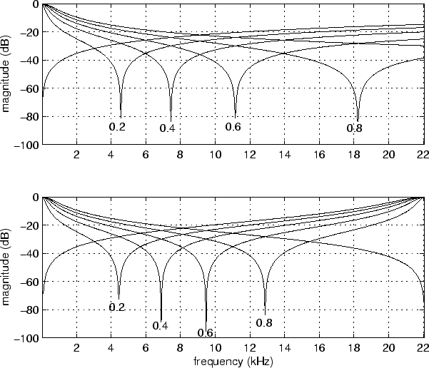As can be expected, the discrete-time model closely approximates the continuous-time model at the lower frequencies. However, the deviation is rather large at the higher frequencies. Fortunately, this discrepancy is relatively insignificant in a full instrument implementation, because the air column reflection function is strongly low-pass due to viscothermal and radiation losses.