Next |
Prev |
Up |
Top
|
Index |
JOS Index |
JOS Pubs |
JOS Home |
Search
The Triangular Scheme
The simplest difference scheme which can be used to solve the wave equation on a triangular grid, and which corresponds to the waveguide mesh discussed in
[2]
in the constant-coefficient case, is given by
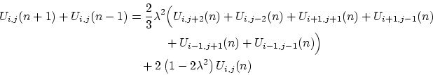 |
(19) |
for a grid defined by points at indices  , for integer
  and
and  such that
  is even. These coordinates refer to grid points at locations
 and
and
 , so that a given grid point is equidistant from its six neighbors. This arrangement is shown in Figure 4(a) and can be considered to be a rectilinear grid under a coordinate transformation; we refer to [9] for a discussion of the range of allowable spatial frequencies for such a grid.
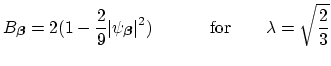
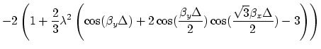
In this case, we will again have an amplification polynomial of the form (5), with
Because
 is not multilinear (see §3.2) in the cosines, finding the extrema is not as simple as in the interpolated case--one can proceed either through some tedious algebra, change to stretched rectilinear coordinates, in which
becomes multilinear again, or make use of a computer. In any case, these extrema can be shown to be
is not multilinear (see §3.2) in the cosines, finding the extrema is not as simple as in the interpolated case--one can proceed either through some tedious algebra, change to stretched rectilinear coordinates, in which
becomes multilinear again, or make use of a computer. In any case, these extrema can be shown to be
and thus, from (9),
This is surprising, because the bound for passivity, from
Eqn. (4.80) of [2],
of the triangular mesh is
 . That is to say,
for a given inter-junction spacing of
. That is to say,
for a given inter-junction spacing of  , a triangular waveguide
mesh
is concretely passive for time steps
, a triangular waveguide
mesh
is concretely passive for time steps  with
with
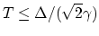 . The corresponding difference
equation, namely (18), is stable (in the sense of Von
Neumann), for
. The corresponding difference
equation, namely (18), is stable (in the sense of Von
Neumann), for
 . The waveguide
mesh can of course operate in a non-passive mode for
. The waveguide
mesh can of course operate in a non-passive mode for
 (where we will require negative
self-loop immittances, and will not have a simple positive definite
energy measure for the network in terms of the wave quantities). The
numerical dispersion characteristics of the scheme at the two bounds
are considerably different, and are plotted in Figure
4(b) and (c); the phase velocities are near the correct
physical velocity over a much wider range of spatial frequencies at
the stability bound, though the dispersion is also more directional.
(where we will require negative
self-loop immittances, and will not have a simple positive definite
energy measure for the network in terms of the wave quantities). The
numerical dispersion characteristics of the scheme at the two bounds
are considerably different, and are plotted in Figure
4(b) and (c); the phase velocities are near the correct
physical velocity over a much wider range of spatial frequencies at
the stability bound, though the dispersion is also more directional.
The question which arises here is of the distinction between passive
and stable numerical methods
(this was also seen for the mesh for the transmission line equations in
the previous section on the interpolated rectilinear scheme). Is it
always possible to find a passive realization of a stable numerical
method? The discussion on the hexagonal mesh will help to answer this
question. To this end, we note that at the stability limit, we can
rewrite
 as
as
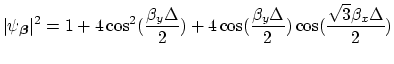
for a function
 whose squared magnitude is given by
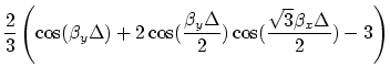
The spectral amplification factors at the stability limit will then be, from (6),
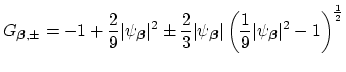 |
(20) |
For
 (its limiting value), the triangular scheme has the same potential for instability as the rectilinear scheme. Linear growth may occur for this scheme at the seven spatial frequency pairs
![\begin{figure}[h]
\begin{center}
\begin{picture}(560,200)
\par
\put(30,10){\ep...
...e}/\gamma$\ at the stability bound, for $\lambda = \sqrt{2/3}$.}}
\end{figure}](img213.png)
The computational and add densities for the triangular scheme in general, and at the stability (
) and passivity bounds (
 ) will be
Here we have taken into account the fact that at the passivity bound, we require one less add per point (in the waveguide mesh implementation, the self-loop disappears). We also mention that the triangular difference scheme is doubly pathological, in the sense that not only do its passivity and stability regimes not coincide (and aside from the interpolated rectilinear schemes, it is the only scheme examined in this appendix that exhibits this behavior), but it also can not be decomposed into even/odd mutually exclusive subschemes, as can all the other schemes to be discussed here (again, excepting the interpolated scheme). It seems reasonable to conjecture that these two ``symptoms'' are related (somehow).
Next |
Prev |
Up |
Top
|
Index |
JOS Index |
JOS Pubs |
JOS Home |
Search
Download vonn.pdf
 for stability