Next |
Prev |
Up |
Top
|
Index |
JOS Index |
JOS Pubs |
JOS Home |
Search
Although the choice of the free parameter  which gives a maximally direction-independent numerical dispersion profile has been made, in the past, through computerized optimization procedures [4], we note here that it is possible to make a theoretical choice as well, based on a Taylor series expansion of the spectrum.
The spectral amplification factors for the interpolated scheme can be written in terms of the function
 , or, equivalently, in terms of the function
 . It should be clear, then, that if
is directionally independent, then so are the amplification factors, and thus the numerical phase velocity (see §2.4) as well. Ideally, we would like
to be a function of the spectral radius
. It should be clear, then, that if
is directionally independent, then so are the amplification factors, and thus the numerical phase velocity (see §2.4) as well. Ideally, we would like
to be a function of the spectral radius


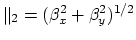 alone. Now examine the Taylor expansion of
about
alone. Now examine the Taylor expansion of
about  :
:
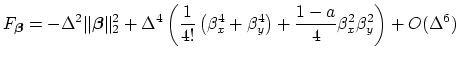
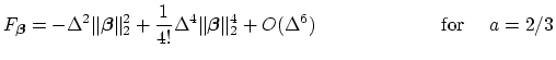
The directionally-independent
 term reflects the fact that the scheme is consistent with the wave equation; higher order terms in general show directional dependence. The choice of
  , however, gives
and the directional dependence is confined to higher-order powers of  . Thus for this choice of , the numerical scheme is maximally direction independent about spatial DC. Note that this value of does fall within the required bounds for a passive waveguide mesh implementation. The value of
  (for which the numerical dispersion profile is plotted in Figure 2), which is very close to
  , was chosen by visual inspection of dispersion profiles for various values of .
Next |
Prev |
Up |
Top
|
Index |
JOS Index |
JOS Pubs |
JOS Home |
Search
Download vonn.pdf