State Space Realization of Second-Order Continuous-Time Lowpass Filters

It is easy to realize a filter transfer function in state-space form by means of the so-called controller-canonical form, in which transfer-function coefficients appear directly in the matrices of the state-space form. In our case, the state-space model becomes

$$\begin{eqnarray*} \underline{\dot{x}}(t) &=& \left[\begin{array}{cc} 0 & 1 \\ [2pt] -a_0 & -a_1 \end{array}\right]\underline{x}(t) + \left[\begin{array}{c} 0 \\ [2pt] 1 \end{array}\right] u(t)\\ [10pt] y(t) &=& \left[\begin{array}{cc} c_0 & c_1 \end{array}\right]\underline{x}(t) \end{eqnarray*}$$

where $a_0=1$ , $a_1=\sqrt{2}$ , $c_0=1$ , and $c_1=0$ for a normalized Butterworth lowpass filter. I.e.,

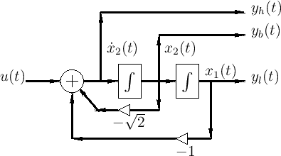
$$\begin{eqnarray*} \dot{x}_1(t) &=& x_2(t)\\ \dot{x}_2(t) &=& -x_1(t) - \sqrt{2}\, x_2(t) + u(t)\\ [10pt] y_l(t) &=& x_1(t). \end{eqnarray*}$$

This system is diagrammed in Fig.3. Note that due to the chain of integrators in controller-canonical form, we also have available the bandpass and highpass outputs as shown in the figure. Each integrator is typically implemented (in analog circuits) by means of an operational amplifier (``op amp'') having a capacitor in its feedback loop.²

Figure 3: State-space realization of second-order normalized Butterworth lowpass filter.