Lossy Finite Difference Recursion

We will now derive a finite-difference model in terms of string displacement samples which correspond to the lossy digital waveguide model of Fig.C.5. This derivation generalizes the lossless case considered in §C.4.3.

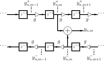
Figure C.7 depicts a digital waveguide section once again in ``physical canonical form,'' as shown earlier in Fig.C.5, and introduces a doubly indexed notation for greater clarity in the derivation below [445,223,124,123].

Figure C.7: Lossy digital waveguide--frequency-independent loss-factors $g$ .

Referring to Fig.C.7, we have the following time-update relations:

$$\begin{eqnarray*} y^{+}_{n+1,m}&=& gy^{+}_{n,m-1}\;=\; g\cdot(y_{n,m-1}- y^{-}_{n,m-1})\\ y^{-}_{n+1,m}&=& gy^{-}_{n,m+1}\;=\; g\cdot(y_{n,m+1}- y^{+}_{n,m+1}) \end{eqnarray*}$$

Adding these equations gives

$$y_{n+1,m} = g\cdot(y_{n,m-1}+y_{n,m+1}) - g\cdot(\underbrace{y^{-}_{n,m-1}}_{gy^{-}_{n-1,m}} + \underbrace{y^{+}_{n,m+1}}_{gy^{+}_{n-1,m}})$$

$$= g\cdot(y_{n,m-1}+y_{n,m+1}) - g^2 y_{n-1,m} \protect$$ (C.31)

This is now in the form of the finite-difference time-domain (FDTD) scheme analyzed in [223]:

$$y_{n+1,m}= g^{+}_my_{n,m-1}+ g^{-}_my_{n,m+1}+ a_my_{n-1,m},$$

with $g^{+}_m= g^{-}_m= g$ , and $a_m= -g^2$ . In [124], it was shown by von Neumann analysis (§D.4) that these parameter choices give rise to a stable finite-difference scheme (§D.2.3), provided $\vert g\vert\leq 1$ . In the present context, we expect stability to follow naturally from starting with a passive digital waveguide model.