Next |
Prev |
Up |
Top
|
Index |
JOS Index |
JOS Pubs |
JOS Home |
Search
Linear Prediction (LP) implicitly computes a spectral envelope that
is well adapted for audio work, provided the order of the predictor is
appropriately chosen. Due to the error minimized by
LP, spectral peaks are emphasized in the envelope, as they are
in the auditory system. (The peak-emphasis of LP is quantified
in (10.10) below.)
The term ``linear prediction'' refers to the process of predicting a
signal sample  based on
  past samples:
 |
(11.4) |
We call
the order of the linear predictor, and
 the prediction coefficients.
The prediction error (or ``innovations
sequence'' [114]) is denoted
the prediction coefficients.
The prediction error (or ``innovations
sequence'' [114]) is denoted  in (10.4),
and it represents all new information entering the signal
in (10.4),
and it represents all new information entering the signal  at time
 . Because the information is new,
is ``unpredictable.''
The predictable component of
contains no new information.
. Because the information is new,
is ``unpredictable.''
The predictable component of
contains no new information.
Taking the z transform of (10.4) yields
 |
(11.5) |
where
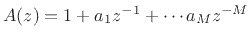 .
In signal modeling by linear prediction, we are given the signal
but not the prediction coefficients
.
In signal modeling by linear prediction, we are given the signal
but not the prediction coefficients  . We must
therefore estimate them. Let
. We must
therefore estimate them. Let
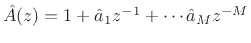 denote the polynomial with estimated prediction
coefficients
denote the polynomial with estimated prediction
coefficients
 . Then we have
 |
(11.6) |
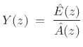
where
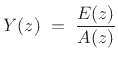
 denotes the estimated prediction-error z transform. By
minimizing
denotes the estimated prediction-error z transform. By
minimizing
 , we define a minimum-least-squares estimate
 . In other words, the linear prediction coefficients
are
defined as those which minimize the sum of squared prediction errors
. In other words, the linear prediction coefficients
are
defined as those which minimize the sum of squared prediction errors

 |
(11.7) |
over some range of
, typically an interval over which the signal
is stationary (defined in Chapter 6). It turns out
that this minimization results in maximally flattening the
prediction-error spectrum  [11,157,162].
That is, the optimal
[11,157,162].
That is, the optimal
 is a whitening filter (also
called an inverse filter). This makes sense in terms
of Chapter 6 when one considers that a flat power spectral
density corresponds to white noise in the time domain, and only white
noise is completely unpredictable from one sample to the next. A
non-flat spectrum corresponds to a nonzero correlation between two
signal samples separated by some nonzero time interval.
is a whitening filter (also
called an inverse filter). This makes sense in terms
of Chapter 6 when one considers that a flat power spectral
density corresponds to white noise in the time domain, and only white
noise is completely unpredictable from one sample to the next. A
non-flat spectrum corresponds to a nonzero correlation between two
signal samples separated by some nonzero time interval.
If the prediction-error is successfully whitened, then the signal
model can be expressed in the frequency domain as
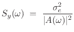 |
(11.8) |
where
 denotes the power spectral density of
(defined
in Chapter 6), and
denotes the power spectral density of
(defined
in Chapter 6), and
 denotes the variance of
the (white-noise) prediction error
. Thus, the spectral
magnitude envelope may be defined as
denotes the variance of
the (white-noise) prediction error
. Thus, the spectral
magnitude envelope may be defined as
EnvelopeLPC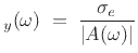 |
(11.9) |
Subsections
Next |
Prev |
Up |
Top
|
Index |
JOS Index |
JOS Pubs |
JOS Home |
Search
[How to cite this work] [Order a printed hardcopy] [Comment on this page via email]