Normalized Scattering Junctions

Figure G.19: The normalized scattering junction.

Using (G.54) to convert to normalized waves $\tilde{f}^\pm$, the Kelly-Lochbaum junction (G.60) becomes

$$\tilde{f}^{+}_i(t) = \sqrt{1-k_i^2(t)} \tilde{f}^{+}_{i-1}(t-T) - k_i(t) \tilde{f}^{-}_i(t)$$

$$\tilde{f}^{-}_{i-1}(t+T) = k_i(t)\tilde{f}^{+}_{i-1}(t-T) + \sqrt{1-k_i^2(t)}\tilde{f}^{-}_i(t)$$ (G.66)

as diagrammed in Fig. G.19. This is called the normalized scattering junction [275], although a more precise term would be the ``normalized-wave scattering junction.''

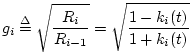
It is interesting to define $\theta_i \isdef \sin^{-1}(k_i)$, always possible for passive junctions since $-1\leq k_i\leq 1$, and note that the normalized scattering junction is equivalent to a 2D rotation:

$$\tilde{f}^{+}_i(t) = \cos(\theta_i) \tilde{f}^{+}_{i-1}(t-T) - \sin(\theta_i) \tilde{f}^{-}_i(t)$$

$$\tilde{f}^{-}_{i-1}(t+T) = \sin(\theta_i)\tilde{f}^{+}_{i-1}(t-T) + \cos(\theta_i)\tilde{f}^{-}_i(t)$$ (G.67)

where, for conciseness of notation, the time-invariant case is written.

While it appears that scattering of normalized waves at a two-port junction requires four multiplies and two additions, it is possible to convert this to three multiplies and three additions using a two-multiply ``transformer'' to power-normalize an ordinary one-multiply junction [408].

The transformer is a lossless two-port defined by [127]

$$f^{{+}}_i(t) = g_i f^{{+}}_{i-1}(t-T)$$

$$f^{{-}}_{i-1}(t+T) = \frac{1}{g_i}f^{{-}}_i(t)$$ (G.68)

The transformer can be thought of as a device which steps the wave impedance to a new value without scattering; instead, the traveling signal power is redistributed among the force and velocity wave variables to satisfy the fundamental relations $f^\pm =\pm Rv^\pm$ (G.57) at the new impedance. An impedance change from $R_{i-1}$ on the left to $R_i$ on the right is accomplished using

$$g_i \isdef \sqrt\frac{R_i}{R_{i-1}} = \sqrt\frac{1-k_i(t)}{1+k_i(t)}$$ (G.69)

as can be quickly derived by requiring $(f^{{+}}_{i-1})^2/R_{i-1}= (f^{{+}}_i)^2/R_i$. The parameter $g_i$ can be interpreted as the ``turns ratio'' since it is the factor by which force is stepped (and the inverse of the velocity step factor).

Figure G.20: The three-multiply normalized scattering junction.

Figure G.20 illustrates the three-multiply normalized scattering junction [408]. The one-multiply junction of Fig. G.18 is normalized by the transformer on its left. Since the impedance discontinuity is created locally by the transformer, all wave variables in the delay elements to the left and right of the overall junction are at the same wave impedance. Thus, using transformers, all waveguides can be normalized to the same impedance, e.g., $R_i\equiv 1$.

It is important to notice that $g_i$ and $1/g_i$ may have a large dynamic range in practice. For example, if $k_i\in [-1+\epsilon,1-\epsilon]$, the transformer coefficients may become as large as $\sqrt{2/\epsilon - 1}$. If $\epsilon$ is the ``machine epsilon,'' i.e., $\epsilon = 2^{-(n-1)}$ for typical $n$-bit two's complement arithmetic normalized to lie in $[-1,1)$, then the dynamic range of the transformer coefficients is bounded by $\sqrt{2^n-1}\approx 2^{n/2}$. Thus, while transformer-normalized junctions trade a multiply for an add, they require up to $50$% more bits of dynamic range within the junction adders.