Equivalence of Parallel Combs to TDLs

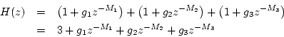
It is easy to show that the TDL of Fig. 1.13 is equivalent to a parallel combination of three feedforward comb filters, each as in Fig. 1.17. To see this, we simply add the three comb-filter transfer functions of Eq. (1.3) and equate coefficients:

$$\begin{eqnarray*} H(z) &=& \left(1+g_1 z^{-M_1}\right) + \left(1+g_2 z^{-M_2}\... ...\right) \\ &=& 3 + g_1 z^{-M_1} + g_2 z^{-M_2} + g_3 z^{-M_3} \end{eqnarray*}$$

which implies

$$b_0 = 3,\; b_{M_1} = g_1,\; b_{M_2} = g_2,\; b_{M_3} = g_3 .$$

We see that parallel comb filters require more delay memory ( $M_1+M_2+M_3$ elements) than the corresponding TDL, which only requires $\max(M_1,M_2,M_3)$ elements.