Next  |  Prev  |  Up  |  Top  |  Index  |  JOS Index  |  JOS Pubs  |  JOS Home  |  Search

Lossy Vibration

The DW and FDTD state-space models are equivalent with respect to 
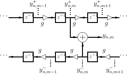
lossy traveling-wave simulation. Figure E.4 shows the flow diagram for the case of simple attenuation by $ g$ per sample of wave propagation, where $ g\in(0,1]$ for a passive string.

Figure E.4: DW flow diagram in the lossy case.
\includegraphics{eps/wglossyCopy}

The DW state update can be written in this case as

$\displaystyle \underline{x}_W(n+2) = g^2\mathbf{A}_W\underline{x}_W(n) + {\mathbf{B}_W}\underline{u}(n+2).
$

where the loss associated with two time steps has been incorporated into the chosen subgrid for physical accuracy. (The neglected subgrid may now be considered lossless.) In changing coordinates to the FDTD scheme, the gain factor $ g^2$ can remain factored out, yielding

$\displaystyle \underline{x}_K(n+2) = g^2\mathbf{A}_K\underline{x}_K(n) + \mathbf{B}_K\underline{u}(n+2).
$

When the input is zero after a particular time, such as in a plucked or struck string simulation, the losses can be implemented at the final output, and only when an output is required, e.g.,

$\displaystyle y(n) = g^n y_0(n)
$

where $ y_0(n)$ denotes the corresponding lossless simulation. When there is a general input signal, the state vector needs to be properly attenuated by losses. In the DW case, the losses can be lumped at two points per spatial input and output [450].


Next  |  Prev  |  Up  |  Top  |  Index  |  JOS Index  |  JOS Pubs  |  JOS Home  |  Search

[How to cite this work]  [Order a printed hardcopy]  [Comment on this page via email]

``Physical Audio Signal Processing'', by Julius O. Smith III, W3K Publishing, 2010, ISBN 978-0-9745607-2-4
Copyright © 2023-08-20 by Julius O. Smith III
Center for Computer Research in Music and Acoustics (CCRMA),   Stanford University
CCRMA