Avoiding Discontinuities When Changing Delay

We have seen examples (e.g., Figures 4.16 and 4.18) of the general fact that every Lagrange interpolator provides an integer delay at frequency $\omega T = \pi$ , except when the interpolator gain is zero at $\omega T = \pi$ . This is true for any interpolator implemented as a real FIR filter, i.e., as a linear combination of signal samples using real coefficients.^5.4Therefore, to avoid a relatively large discontinuity in phase delay (at high frequencies) when varying the delay over time, the requested interpolation delay should stay within a half-sample range of some fixed integer, irrespective of interpolation order. This provides that the requested delay stays within the ``capture zone'' of a single integer at half the sampling rate. Of course, if the delay varies by more than one sample, there is no way to avoid the high-frequency discontinuity in the phase delay using Lagrange interpolation.

Even-order Lagrange interpolators have an integer at the midpoint of their central one-sample range, so they spontaneously offer a one-sample variable delay free of high-frequency discontinuities.

Odd-order Lagrange interpolators, on the other hand, must be shifted by $1/2$ sample in either direction in order to be centered about an integer delay. This can result in stability problems if the interpolator is used in a feedback loop, because the interpolation gain can exceed 1 at some frequency when venturing outside the central one-sample range (see §4.2.11 below).

In summary, discontinuity-free interpolation ranges include

$$\begin{eqnarray*} \frac{N}{2}-\frac{1}{2} < D < \frac{N}{2}+\frac{1}{2}&& \mbox{($N$\ even)},\\ \frac{N+1}{2}-\frac{1}{2} < D < \frac{N+1}{2}+\frac{1}{2}&& \mbox{($N$\ odd).} \end{eqnarray*}$$

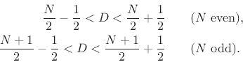
Wider delay ranges, and delay ranges not centered about an integer delay, will include a phase discontinuity in the delay response (as a function of delay) which is largest at frequency $\omega T = \pi$ , as seen in Figures 4.16 and 4.18.