Multivariable Formulation of the Waveguide

Perhaps the most straightforward multivariable generalization of (2) and (3) is

$$\displaystyle \frac{\partial {\mbox{\boldmath$p$}}({\mbox{\boldmath$x$}},t)}{\partial {\mbox{\boldmath$x$}}} = - {\mbox{\boldmath$M$}}\frac{\partial {\mbox{\boldmath$u$}}({\mbox{\boldmath$x$}},t)}{\partial t}$$ (5)

$$\displaystyle % needed for each line \frac{\partial {\mbox{\boldmath$p$}}({\mbox{\boldmath$x$}},t)}{\partial t} = - {\mbox{\boldmath$K$}}\frac{\partial {\mbox{\boldmath$u$}}({\mbox{\boldmath$x$}},t)}{\partial {\mbox{\boldmath$x$}}}$$ (6)

in the spatial coordinates ${\mbox{\boldmath$x$}}^T \stackrel{\triangle}{=}[x_1\,\cdots\,x_m]$ at time $t$, where ${\mbox{\boldmath$M$}}$ and ${\mbox{\boldmath$K$}}$ are $m \times m$ non-singular matrices playing the respective roles of multidimensional mass and tension. Differentiating (5) with respect to ${\mbox{\boldmath$x$}}$ and (6) with respect to $t$, and eliminating the term $\partial^2 {\mbox{\boldmath$u$}}({\mbox{\boldmath$x$}},t)/\partial {\mbox{\boldmath$x$}}\partial t$ yields the $m$-variable generalization of the wave equation

$$\frac{\partial^2 {\mbox{\boldmath$p$}}({\mbox{\boldmath$x$}}... ...({\mbox{\boldmath$x$}},t)}{\partial {\mbox{\boldmath$x$}}^2} .$$ (7)

The second spatial derivative is defined here as

$$\left[ \frac{\partial^2{\mbox{\boldmath$p$}}({\mbox{\boldmat... ...ox{\boldmath$x$}},t)}{\partial x_m^2} \end{array}\right] \,.$$ (8)

Similarly, differentiating (5) with respect to $t$ and (6) with respect to ${\mbox{\boldmath$x$}}$, and eliminating $\partial^2{\mbox{\boldmath$p$}}({\mbox{\boldmath$x$}},t)/\partial {\mbox{\boldmath$x$}}\partial t$ yields

$$\frac{\partial^2 {\mbox{\boldmath$u$}}({\mbox{\boldmath$x$}}... ...({\mbox{\boldmath$x$}},t)}{\partial {\mbox{\boldmath$x$}}^2} .$$ (9)

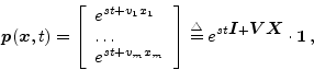
For digital waveguide modeling, we desire solutions of the multivariable wave equation involving only sums of traveling waves. Consider the eigenfunction

$${\mbox{\boldmath$p$}}({\mbox{\boldmath$x$}},t) = \left[ \begi... ...math$V$}}{\mbox{\boldmath$X$}}} \cdot {\mbox{\boldmath$1$}}\,,$$ (10)

where $s$ is interpreted as a Laplace-transform variable $s=\sigma+j\omega$, ${\mbox{\boldmath$I$}}$ is the $m \times m$ identity matrix, ${\mbox{\boldmath$X$}}{\tiny\stackrel{\triangle}{=}} \hbox{diag}({\mbox{\boldmath$x$}})$, ${\mbox{\boldmath$V$}}{\tiny\stackrel{\triangle}{=}}\hbox{diag}([v_1, \ldots, v_m])$ is a diagonal matrix of spatial Laplace-transform variables (the imaginary part of $v_i$ being spatial frequency along the $i$th spatial coordinate), and ${\mbox{\boldmath$1$}}^T {\tiny\stackrel{\triangle}{=}}[1, \ldots, 1]$ is the $m$-dimensional vector of ones. Applying the eigenfunction (10) to (7) gives the algebraic equation

$$s^2{\mbox{\boldmath$I$}}= {\mbox{\boldmath$K$}}{\mbox{\boldm... ...angle}{=}{\mbox{\boldmath$C_p$}}^2 {\mbox{\boldmath$V$}}^2 \,,$$ (11)

where ${\mbox{\boldmath$C_p$}}$ is the diagonal matrix of sound-speeds along the $m$ coordinate axes. Since ${\mbox{\boldmath$C_p$}}^2{\mbox{\boldmath$V$}}^2 = s^2{\mbox{\boldmath$I$}}$, we have

$${\mbox{\boldmath$V$}}=\pm s {\mbox{\boldmath$C_p$}}^{-1} \,.$$ (12)

Substituting (12) into (10), the eigensolutions of (7) are found to be of the form

$${\mbox{\boldmath$p$}}({\mbox{\boldmath$x$}}, t) = e^{s\left(... ...1}{\mbox{\boldmath$X$}}\right)} \cdot {\mbox{\boldmath$1$}}\,.$$ (13)

Similarly, applying (10) to (9) yields

$${\mbox{\boldmath$V$}}=\pm s {\mbox{\boldmath$C_u$}}^{-1} \,,$$ (14)

where ${\mbox{\boldmath$C_u$}}\stackrel{\triangle}{=}{\mbox{\boldmath$M$}}^{-1}{\mbox{\boldmath$K$}}$. The eigensolutions of (9) are then of the form

$${\mbox{\boldmath$u$}}({\mbox{\boldmath$x$}}, t) = e^{s\left(... ...1}{\mbox{\boldmath$X$}}\right)} \cdot {\mbox{\boldmath$1$}}\,.$$ (15)

The generalized sound-speed matrices ${\mbox{\boldmath$C_p$}}$ and ${\mbox{\boldmath$C_u$}}$ are the same whenever ${\mbox{\boldmath$M$}}^{-1}$ and ${\mbox{\boldmath$K$}}$ commute, e.g., when they are both diagonal.

Having established that (13) is a solution of (7) when condition (11) holds on the matrices ${\mbox{\boldmath$M$}}$ and ${\mbox{\boldmath$K$}}$, we can express the general traveling-wave solution to (7) in both pressure and velocity as

$$\begin{array}{l} {\mbox{\boldmath$p$}}({\mbox{\boldmath$x$}... ...\mbox{\boldmath$u$}}^++ {\mbox{\boldmath$u$}}^-\,, \end{array}$$ (16)

where ${\mbox{\boldmath$p$}}^+{\tiny\stackrel{\triangle}{=}}{\bf f}(t{\mbox{\boldmath$I$}}-{\mbox{\boldmath$C_p$}}^{-1}{\mbox{\boldmath$X$}})$, and ${\bf f}$ is an arbitrary superposition of right-going components of the form (13) (i.e., taking the minus sign), and ${\mbox{\boldmath$p$}}^-{\tiny\stackrel{\triangle}{=}} {\bf g}(t{\mbox{\boldmath$I$}}+{\mbox{\boldmath$C_p$}}^{-1}{\mbox{\boldmath$X$}})$ is similarly any linear combination of left-going eigensolutions from (13) (all having the plus sign). Similar definitions apply for ${\mbox{\boldmath$u$}}^+$ and ${\mbox{\boldmath$u$}}^-$. When the time and space arguments are dropped as in the right-hand side of (16), it is understood that all the quantities are written for the same time $t$ and position ${\mbox{\boldmath$x$}}$.

When the mass and tension matrices ${\mbox{\boldmath$M$}}$ and ${\mbox{\boldmath$K$}}$ are diagonal, our analysis corresponds to considering $m$ separate waveguides as a whole. For example, the two transversal planes of vibration in a string can be described by (7) with $m=2$. In a musical instrument such as the piano [29], the coupling among the strings and between different vibration modalities within a single string, occurs primarily at the bridge [30]. Indeed, the bridge acts like a junction of several multivariable waveguides (see section IV).

When the matrices ${\mbox{\boldmath$M$}}$ and ${\mbox{\boldmath$K$}}$ are non-diagonal, the physical interpretation can be of the form

$${{\mbox{\boldmath$C_p$}}}^2\stackrel{\triangle}{=}{\mbox{\boldmath$K$}}{\mbox{\boldmath$M$}}^{-1} \,,$$ (17)

where ${\mbox{\boldmath$K$}}$ is the stiffness matrix, and ${\mbox{\boldmath$M$}}$ is the mass density matrix. ${\mbox{\boldmath$C_p$}}$ is diagonal if (11) holds, and in this case, the wave equation (7) is decoupled in the spatial dimensions. There are physical examples where the matrices ${\mbox{\boldmath$M$}}$ and ${\mbox{\boldmath$K$}}$ are not diagonal, even though (17) is satisfied with a diagonal ${\mbox{\boldmath$C_p$}}$. One such example, in the domain of electrical variables, is given by $m$ conductors in a sheath or above a ground plane, where the sheath or the ground plane acts as a coupling element [31, pp. 67-68]. In acoustics, it is more common to have coupling introduced by a dissipative term in equation (7), but the solution can still be expressed as decoupled attenuating traveling waves. An example of such acoustical systems will be presented in Section III-B.

Besides the existence of physical systems that support multivariable traveling wave solutions, there are other practical reasons for considering a multivariable formulation of wave propagation. For instance, modal analysis considers the vector ${\mbox{\boldmath$p$}}$ (whose dimension is infinite in general) of coefficients of the normal mode expansion of the system response. For spaces in perfectly reflecting enclosures, ${\mbox{\boldmath$p$}}$ can be compacted so that each element accounts for all the modes sharing the same spatial dimension [32]. ${\mbox{\boldmath$p$}}$ admits a wave decomposition as in (16), and ${\mbox{\boldmath$C_p$}}$ is diagonal. Having walls with finite impedance, there is a damping term proportional to $\partial {\mbox{\boldmath$p$}}/\partial t$ that functions as a coupling term among the ideal modes [33]. Coupling among the modes can also be exerted by diffusive properties of the enclosure [32,9].

Note that the multivariable wave equation (7) considered here does not include wave equations governing propagation in multidimensional media (such as membranes, spaces, and solids). In higher dimensions, the solution in the ideal linear lossless case is a superposition of waves traveling in all directions in the $m$-dimensional space [27]. However, it turns out that a good simulation of wave propagation in a multidimensional medium may in fact be obtained by forming a mesh of unidirectional waveguides as considered here, each described by (7); such a mesh of 1D waveguides can be shown to solve numerically a discretized wave equation for multidimensional media [34,35,13,14].