It is quite common to want to vary the resonance frequency of a resonator in real time. This is a special case of a tunable filter. In the pre-digital days of analog synthesizers, filter modules were tuned by means of control voltages, and were thus called voltage-controlled filters (VCF). In the digital domain, control voltages are replaced by time-varying filter coefficients. In the time-varying case, the choice of filter structure has a profound effect on how the filter characteristics vary with respect to coefficient variations. In this section, we will take a look at the time-varying two-pole resonator.
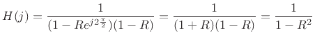
Evaluating the transfer function of the two-pole resonator
(Eq.(B.1)) at the point
![]() on the unit circle
(the filter's resonance frequency
on the unit circle
(the filter's resonance frequency
![]() ) yields a gain at resonance equal to
) yields a gain at resonance equal to
In the middle frequency between dc and
and, since
An important fact we can now see is that the gain at resonance depends markedly on the resonance frequency. In particular, the ratio of the two cases just analyzed is
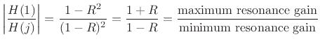
We did not show that resonance gain is maximized at
Note that the ratio of the dc resonance gain to the ![]() resonance
gain is unbounded! The sharper the resonance (the closer
resonance
gain is unbounded! The sharper the resonance (the closer ![]() is to 1), the greater the disparity in the gain.
is to 1), the greater the disparity in the gain.
Figure B.17 illustrates a number of resonator frequency responses
for the case ![]() . (Resonators in practice may use values of
. (Resonators in practice may use values of ![]() even closer to 1 than this--even the case
even closer to 1 than this--even the case ![]() is used for making
recursive digital sinusoidal oscillators [90].) For
resonator tunings at dc and
is used for making
recursive digital sinusoidal oscillators [90].) For
resonator tunings at dc and ![]() , we predict the resonance gain to
be
, we predict the resonance gain to
be
![]() dB, and this is what we see in the plot.
When the resonance is tuned to
dB, and this is what we see in the plot.
When the resonance is tuned to ![]() , the gain drops well below 40
dB. Clearly, we will need to compensate this gain variation when
trying to use the two-pole digital resonator as a tunable filter.
, the gain drops well below 40
dB. Clearly, we will need to compensate this gain variation when
trying to use the two-pole digital resonator as a tunable filter.
![\includegraphics[width=\twidth ]{eps/resgain}](img1521.png) |
Figure B.18 shows the same type of plot for the complex
one-pole resonator
![]() , for
, for ![]() and
10 values of
and
10 values of ![]() . In this case, we expect the frequency
response evaluated at the center frequency to be
. In this case, we expect the frequency
response evaluated at the center frequency to be
![]() . Thus, the gain at
resonance for the plotted example is
. Thus, the gain at
resonance for the plotted example is
![]() db for all
tunings. Furthermore, for the complex resonator, the resonance gain
is also exactly equal to the peak gain.
db for all
tunings. Furthermore, for the complex resonator, the resonance gain
is also exactly equal to the peak gain.
![\includegraphics[width=\twidth ]{eps/cresgain}](img1524.png) |