IIR Example

Figure 5.8 plots an IIR filter example for the filter

$$y(n) = x(n) + 0.99\, y(n-1).$$

The previous matlab is modified as follows:

      Nh = 300; % APPROXIMATE filter length (visually in plot)
      B = 1; A = [1 -0.99]; % One-pole recursive example
      ...       % otherwise as above for the FIR example

The decay time for this recursive filter was arbitrarily marked at 300 samples (about three time-constants of decay).

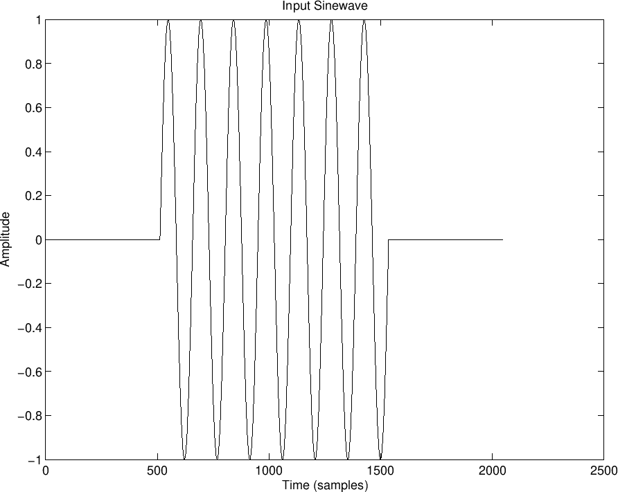
Figure 5.8: Example transient, steady-state, and decay responses for an IIR ``one-pole'' filter driven by a gated sinusoid.

Input Signal

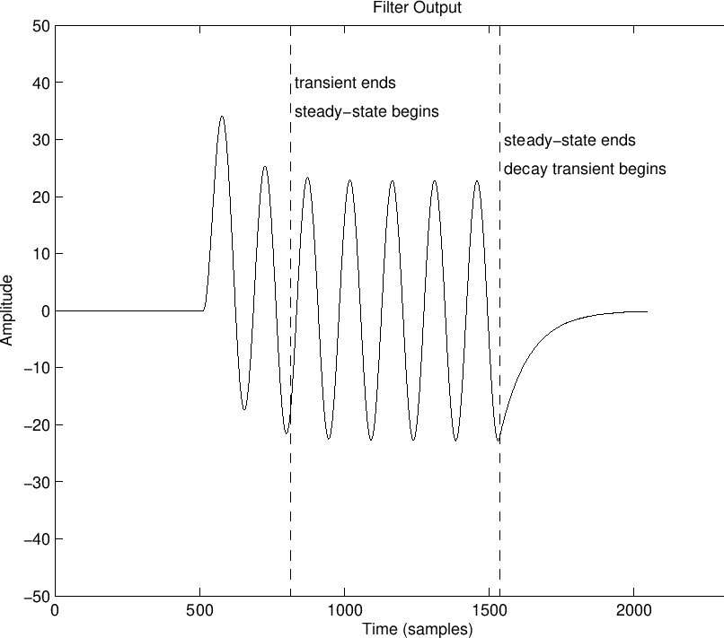
Filter Output Signal