Parallel Case

Figure 6.2: Parallel combination of transfer functions $H_1(z)$ and $H_2(z)$, yielding $H(z)=H_1(z)+H_2(z)$.

Figure 6.2 illustrates the parallel combination of two filters. The filters $H_1(z)$ and $H_2(z)$ are driven by the same input signal $x(n)$, and their respective outputs $y_1(n)$ and $y_2(n)$ are summed. The transfer function of the parallel combination is therefore

$$H(z) \isdefs \frac{Y(z)}{X(z)} \eqsp \frac{Y_1(z) + Y_2(z)}{X(z)} \eqsp \frac{Y_1(z)}{X(z)} + \frac{Y_2(z)}{X(z)} \isdefs H_1(z)+H_2(z).$$

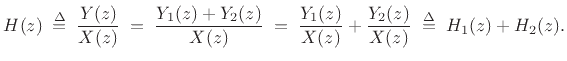
where we needed only linearity of the z transform to have that ${\cal Z}\{y_1+y_2\} = {\cal Z}\{y_1\}+{\cal Z}\{y_2\}$.