Next |
Prev |
Up |
Top
|
Index |
JOS Index |
JOS Pubs |
JOS Home |
Search
The phase response is almost as easy to evaluate graphically as is the
amplitude response:
If  is real, then
  is either 0 or
  . Terms of the
form
. Terms of the
form
 can be interpreted as a vector drawn from the point
  to the point
 in the complex plane. The angle of
is
the angle of the constructed vector (where a vector pointing
horizontally to the right has an angle of 0). Therefore, the phase
response at frequency
in the complex plane. The angle of
is
the angle of the constructed vector (where a vector pointing
horizontally to the right has an angle of 0). Therefore, the phase
response at frequency  Hz is again obtained by drawing lines from
all the poles and zeros to the point
Hz is again obtained by drawing lines from
all the poles and zeros to the point
 , as shown in
Fig.8.4. The angles of the lines from the zeros are added, and
the angles of the lines from the poles are subtracted. Thus, at the
frequency
, as shown in
Fig.8.4. The angles of the lines from the zeros are added, and
the angles of the lines from the poles are subtracted. Thus, at the
frequency  the phase response of the two-pole two-zero filter
in the figure is
the phase response of the two-pole two-zero filter
in the figure is
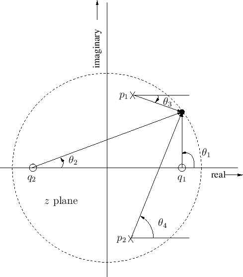 .
.
Figure 8.4:
Measurement of phase response from a pole-zero diagram.
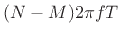 |
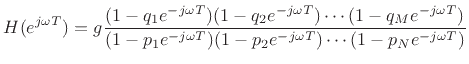
Note that an additional phase of
 radians appears when
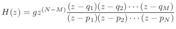
the number of poles is not equal to the number of zeros. This factor
comes from writing the transfer function as
radians appears when
the number of poles is not equal to the number of zeros. This factor
comes from writing the transfer function as
and may be thought of as arising from  additional zeros at
  when
when  , or
, or 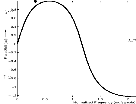 poles at
when
poles at
when  . Strictly
speaking, every digital filter has an equal number of poles and zeros
when those at
and
. Strictly
speaking, every digital filter has an equal number of poles and zeros
when those at
and
 are counted. It is customary,
however, when discussing the number of poles and zeros a filter has,
to neglect these, since they correspond to pure delay and do not
affect the amplitude response. Figure 8.5 gives the phase
response for this two-pole two-zero example.
are counted. It is customary,
however, when discussing the number of poles and zeros a filter has,
to neglect these, since they correspond to pure delay and do not
affect the amplitude response. Figure 8.5 gives the phase
response for this two-pole two-zero example.
Figure 8.5:
Phase response obtained from Fig.8.4
for positive frequencies. The point of the phase response
corresponding to the arrows in that figure is marked by a heavy
dot. For real filters, the phase response is
odd (
 ), so the curve
shown here may be reflected through 0 and negated
to obtain the plot for negative frequencies.
), so the curve
shown here may be reflected through 0 and negated
to obtain the plot for negative frequencies.
 |
Next |
Prev |
Up |
Top
|
Index |
JOS Index |
JOS Pubs |
JOS Home |
Search
[How to cite this work] [Order a printed hardcopy] [Comment on this page via email]

