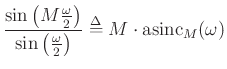
Next  |  Top  |  JOS Index  |  JOS Pubs  |  JOS Home  |  Search

The Rectangular Window

Previously, we looked at the rectangular window:

$\displaystyle w_R(n) \mathrel{\stackrel{\mathrm{\Delta}}{=}}\left\{\begin{array}{ll}
1, & \left\vert n\right\vert\leq\frac{M-1}{2} \\ [5pt]
0, & \hbox{otherwise} \\
\end{array} \right.
$

\epsfig{file=eps/rectWindow.eps,width=5in}

The window transform (DTFT) was found to be

$\displaystyle W_R(\omega)$ $\displaystyle =$ $\displaystyle \frac{\sin\left(M\frac{\omega}{2}\right)}{\sin\left(\frac{\omega}{2}\right)}
\mathrel{\stackrel{\mathrm{\Delta}}{=}}M\cdot \hbox{asinc}_M(\omega)$ (1)

where $ \hbox{asinc}_M(\omega)$ denotes the aliased sinc function.

$\displaystyle \hbox{asinc}_M(\omega) \mathrel{\stackrel{\mathrm{\Delta}}{=}}\frac{\sin(M\omega/2)}{M\cdot \sin(\omega/2)}
$

This result is plotted below:

\epsfig{file=eps/rectWindowRawFT.eps,width=6in,height=3in}

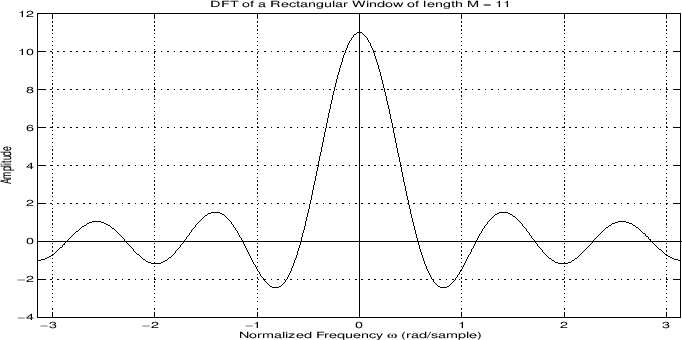
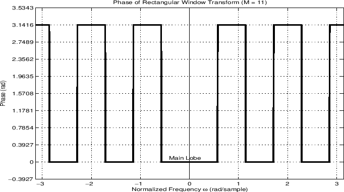
Note that this is the complete window transform, not just its magnitude. We obtain real window transforms like this only for symmetric, zero-centered windows.

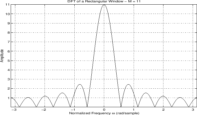
More generally, we may plot both the magnitude and phase of the window versus frequency:


\begin{psfrags}\psfrag{freq}{ \footnotesize $ \omega / \Omega_M $\ }\begin{center}
\epsfig{file=eps/rectWindowFTzeroX.eps,width=6in,height=3.5in} \\
\end{center} % was epsfbox
\end{psfrags}


\begin{psfrags}\psfrag{freq}{ \footnotesize $ \omega / \Omega_M $\ }\begin{center}
\epsfig{file=eps/rectWindowPhaseFT.eps,width=6in,height=3.5in} \\
\end{center} % was epsfbox
\end{psfrags}

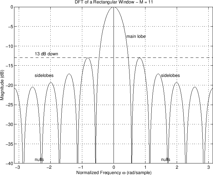
In audio work, we more typically plot the window transform magnitude on a decibel (dB) scale:


\begin{psfrags}\psfrag{freq}{$\omega T$\ (radians per sample)}\begin{center}
\epsfig{file=eps/rectWindowFT.eps,width=6in} \\
\end{center}
\end{psfrags}

Since the DTFT of the rectangular window approximates the sinc function, it should ``roll off'' at approximately 6 dB per octave, as verified in the log-log plot below:


\begin{psfrags}\psfrag{freq}{$\omega T$\ (radians per sample)}\begin{center}
\epsfig{file=eps/rectWindowLLFT.eps,width=6in} \\
\end{center}
\end{psfrags}

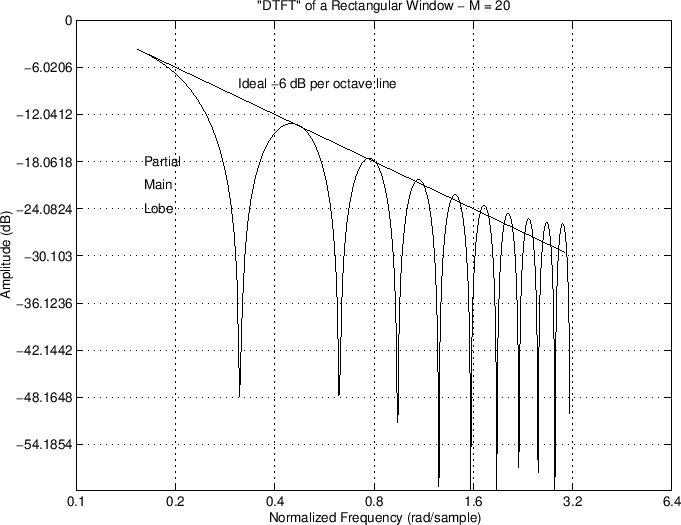
As the sampling rate approaches infinity, the rectangular window transform converges exactly to the sinc function. Therefore, the departure of the roll-off from that of the sinc function can be ascribed to aliasing in the frequency domain, due to sampling in the time domain.


Subsections
Next  |  Top  |  JOS Index  |  JOS Pubs  |  JOS Home  |  Search

[Comment on this page via email]

``FFT Windows'', by Julius O. Smith III and Bill Putnam, (From Lecture Overheads, Music 421).
Copyright © 2020-06-27 by Julius O. Smith III and Bill Putnam
Center for Computer Research in Music and Acoustics (CCRMA),   Stanford University
CCRMA  [Automatic-links disclaimer]