Next |
Top
|
JOS Index |
JOS Pubs |
JOS Home |
Search
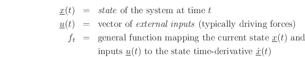
Equations of motion for any physical system
may be conveniently
formulated in terms of its state
 :
:
where
- The function
 may be time-varying, in general
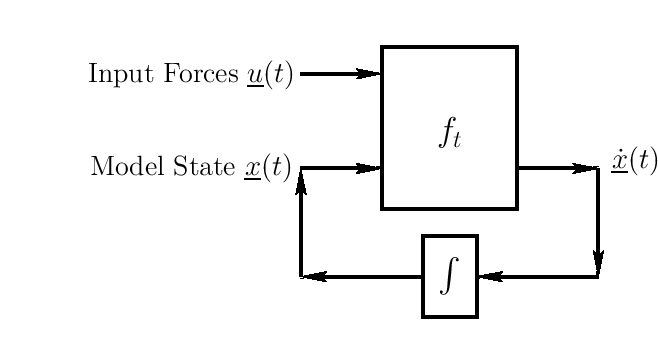
- This potentially nonlinear time-varying model is extremely
general (but causal)
- Even the human brain can be modeled in this form
Subsections
Next |
Top
|
JOS Index |
JOS Pubs |
JOS Home |
Search
Download StateSpace.pdf
Download StateSpace_2up.pdf
Download StateSpace_4up.pdf