If we are interested in using a grid of doubled density over a particular region of the problem domain (in order to surround a particular feature or an irregular part of the boundary), then we are faced with corners, and must develop special scattering junctions for them. An example of an irregular partitioning of the problem domain into two regions, ![]() and
and ![]() , is shown in Figure 4.36(a).
, is shown in Figure 4.36(a).
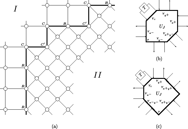 |
There are two types of corners which can arise in an irregular domain decomposition of this kind: those which are concave with respect to region ![]() (the grid point at such a corner is labelled
(the grid point at such a corner is labelled ![]() in Figure 4.36(a)), and those which are concave with respect to region
in Figure 4.36(a)), and those which are concave with respect to region ![]() (labelled
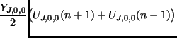
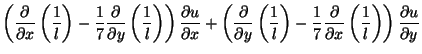
(labelled ![]() ). There are obviously four possible orientations for each type of corner, though, by symmetry, we need only treat the type shown. Because the admittances of the boundary waveguides (represented by thick lines connecting boundary points) are now prescribed, then for a corner junction the linking admittances are fixed; only the self-loop admittance may be varied. Scattering junctions corresponding to corners of type
). There are obviously four possible orientations for each type of corner, though, by symmetry, we need only treat the type shown. Because the admittances of the boundary waveguides (represented by thick lines connecting boundary points) are now prescribed, then for a corner junction the linking admittances are fixed; only the self-loop admittance may be varied. Scattering junctions corresponding to corners of type ![]() and
and ![]() are shown in Figure 4.36(b) and (c).
are shown in Figure 4.36(b) and (c).
Suppose we have a corner point of type ![]() located at coordinates
located at coordinates ![]() . Then, from the results previously given in this section, the admittances of the five waveguides connecting this corner to its neighbors will be
. Then, from the results previously given in this section, the admittances of the five waveguides connecting this corner to its neighbors will be
 |
||||
 |
 |
|||
 |
The corner junction is, however, still lossless, as are all junctions in this waveguide network, and hence a simulation of the parallel-plate system using such a mesh will be stable, regardless of inconsistencies at the corners. It is possible to argue, loosely speaking, that if the number of corners in the interface does not grow as the grid spacing is decreased (an example of this would be an enclosed rectangular doubled density grid, for which the number of corners will be four, independently of the grid spacing), then the error at the corners will become negligible. Although we will make no attempt to prove this, the simulation which we will present later in this section concurs readily with this assertion; indeed, in all tests we have run, any anomalous scattering at the corners is certainly far less important than the first-order scattering error (i.e., numerical reflection) along the interface itself.
In the interest, however, of making any scattering error at the corner junctions as small as possible, we should set, at a corner with coordinates ![]() (in order that the wave speed at the corner is correct, in a gross sense)
(in order that the wave speed at the corner is correct, in a gross sense)
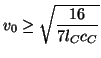 |
A similar argument follows for points ![]() , and we also ideally have
, and we also ideally have ![]() constant in the neighborhood of such points. The setting of the self-loop admittance
constant in the neighborhood of such points. The setting of the self-loop admittance ![]() should be
should be
 |