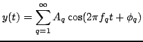
System complexity is, of course, very difficult to define. Perhaps most amenable to discussions of complexity are linear and time-invariant (LTI) systems, which form a starting point for many models of musical instruments. Consider any lossless distributed LTI system (such as a string, bar, membrane, plate, or acoustic tube), freely vibrating at low amplitude due to some set of initial conditions, without any external excitation. Considering the continuous case, one is usually interested in reading an output ![]() from a single location on the object. This solution can almost always be written in the form:
from a single location on the object. This solution can almost always be written in the form:
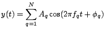
Physical modeling algorithms generally produce sound output at a given sample rate, say ![]() . This is true of all the methods discussed in the previous section. There is thus no hope of (and no need for) simulating frequency components1.1 which lie above
. This is true of all the methods discussed in the previous section. There is thus no hope of (and no need for) simulating frequency components1.1 which lie above ![]() . Thus, as a prelude to a discrete time implementation, the representation (1.8) may be truncated to
. Thus, as a prelude to a discrete time implementation, the representation (1.8) may be truncated to
Even for a vaguely defined system such as this, from this information one may go slightly farther and calculate both the operation count and memory requirements, assuming a modal-type synthesis strategy. As described in §1.2.2, each frequency component in the expression (1.8) may be computed using a single two-pole digital oscillator, which requires two adds, one multiply, and two memory locations, giving, thus, ![]() adds and
adds and ![]() multiplies per time step, and a necessary
multiplies per time step, and a necessary ![]() units of memory. Clearly if fewer than
units of memory. Clearly if fewer than ![]() oscillators are employed, the resulting simulation will not be complete, and the use of more than
oscillators are employed, the resulting simulation will not be complete, and the use of more than ![]() oscillators is superfluous. Not surprisingly, such a measure of complexity is not restricted to frequency domain methods only; in fact, any method (including direct simulation methods such as finite differences and finite element methods) for computing the solution to such a system must require roughly the same amount of memory and number of operations; for time domain methods, complexity is intimately related to conditions for numerical stability. Much more will be said about this in Chapter 6, which deals with time domain and modal solutions for the wave equation.
oscillators is superfluous. Not surprisingly, such a measure of complexity is not restricted to frequency domain methods only; in fact, any method (including direct simulation methods such as finite differences and finite element methods) for computing the solution to such a system must require roughly the same amount of memory and number of operations; for time domain methods, complexity is intimately related to conditions for numerical stability. Much more will be said about this in Chapter 6, which deals with time domain and modal solutions for the wave equation.
There is, however, at least one very interesting exception to this rule. Consider the special case of a system for which the modal frequencies are multiples of a common frequency ![]() , i.e., in (1.8),
, i.e., in (1.8),
![]() . Clearly, then, in this case, (1.8) is a Fourier series representation of a periodic waveform, of period
. Clearly, then, in this case, (1.8) is a Fourier series representation of a periodic waveform, of period ![]() , or, in other words,
, or, in other words,
| (1.9) |
For distributed nonlinear systems, such as strings and percussion instruments, it is difficult to even approach a definition of complexity--perhaps the only thing one can say is that for a given nonlinear system, which reduces to a linear system at low vibration amplitudes (this is the usual case in most of physics, and musical acoustics in particular), the complexity, or required operation count and memory requirements for an algorithm simulating the nonlinear system will be at least that of the associated linear system. Efficiency gains through digital waveguide techniques are no longer possible, except under very restricted conditions--one of these, the string under a tension-modulated nonlinearity, will be discussed in §8.1.5.
One question that will not be approached in detail in this book is of model complexity in the perceptual sense. This is clearly a very important issue, in that psychoacoustic considerations could lead to reductions in both the operation count and memory requirements of a synthesis algorithm, in much the same way as they have impacted on audio compression. For instance, the description of the complexity of a linear system in terms of the number of modal frequencies up to the Nyquist frequency is mathematically sound, but for many musical systems (particularly in 2D), the modal frequencies become very closely spaced in the upper range of the audio spectrum. Taking into consideration the concepts of the critical band and frequency domain masking, it may not be necessary to render the totality of the components. Such psychoacoustic model reduction techniques have been used, with great success, in many efficient (though admittedly non-physical) artificial reverberation algorithms. The impact of psychoacoustics on physical models of musical instruments has seen some investigation recently by Järveläinen [110], in the case of string inharmonicity , and Aramaki [6], in the case of impact sounds, and it would be extremely useful to develop practical complexity-reducing principles and methods, which could be directly related to numerical techniques.
This main point of this section is to signal to the reader that for general systems, there is not a physical modeling synthesis method which acts as a magic bullet. There is a minimum price to be paid for the proper simulation of any system. For a given system, the operation counts for modal, finite difference and lumped network models are always nearly the same; in terms of memory requirements, modal synthesis methods are generally much heavier than for time domain methods. One great misconception which has appeared time and time again in the literature [34] is that time domain methods are wasteful, in the sense that the entire state of an object must be updated, even though one is interested, ultimately, in only a scalar output, generally from a single location on the virtual instrument. Thus point-to-point ``black-box" type models, perhaps based on a transfer function representation are more efficient. But, as will be shown repeatedly throughout this book, the order of any transfer function description (and thus the memory requirements) will be roughly the same as the size of the physical state of the object in question.