Digital waveguides and related scattering methods, as well as modal techniques have undeniably become a very popular means of designing physical modeling sound synthesis algorithms. There are several reasons for this, but the main one is that such structures, built from delay lines and digital filters, Fourier decompositions, fit naturally into the framework of digital signal processing, and form a natural extension of more abstract techniques from the pre-physical modeling synthesis era--note, for instance, the direct link between modal synthesis and additive synthesis, as well as that between digital waveguides and wavetable synthesis, via the Karplus Strong algorithm. Such a body of techniques, with linear system theory at its heart, is home turf to the trained audio engineer.
For some time, however, a separate body of work in the simulation of musical instruments has grown; this work, more often than not, has been carried out by musical acousticians whose primary interest is not so much synthesis, but rather the pure study of the behaviour of musical instruments, often with an eye towards comparison between a model equation and measured data, and possibly potential applications towards improved instrument design. The techniques used by such researchers are of a very different origin, and are couched in a distinct language; as will be seen throughout the rest of this book, however, there is no shortage of links to be made with more standard physical modeling sound synthesis techniques, provided one takes the time to ``translate" between the sets of terminology! In this case, one speaks of time-stepping, and grid resolution; there is no reference to delays or digital filters, and sometimes, the frequency domain is not invoked at all, which is unheard of in the more standard physical modeling sound synthesis setting.
Perhaps the most straightforward approach makes use of a finite difference approximation to a set of partial differential equations [210,102,171], which serves as a mathematical model of a musical instrument. (When applied to dynamic, or time-dependent systems, such techniques are sometimes referred to as ``finite difference time domain" (FDTD) methods, a terminology which originated in numerical methods for the simulation of electromagnetics [215,246,216].) Such methods have a very long history in applied mathematics, which can be traced back at least as far as the work of Courant, Friedrichs and Lewy in 1928 [61], especially as applied to the simulation of fluid dynamics [106] and electromagnetics [215]. Needless to say, the literature on finite difference methods is vast. As mentioned above, they have been applied for some time for sound synthesis purposes, though definitely without the success or widespread acceptance of methods such as digital waveguides, primarily because of computational cost--or, rather, preconceived notions about computational cost.
|
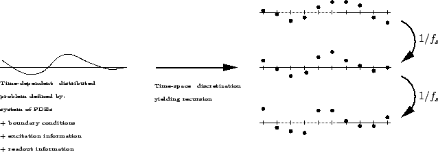
The procedure, which is similar across all types of systems, is very simply described: the spatial domain of a continuous system, described by some model PDE, is restricted to a grid composed of a finite set of points (see Figure 1.12), at which values of a numerical solution are computed. Time is similarly discretized, and the numerical solution is advanced, through a recursion derived from the model PDE. Derivatives are approximated by differences among values at nearby grid points. The great advantage of finite difference methods (among other time domain techniques), in comparison with all the other methods discussed here, is their generality and simplicity, and the wide range of systems to which they may be applied, including strongly nonlinear distributed systems; these can not be approached using waveguides or modal synthesis, and by lumped models only in a very ad hoc and non-rigorous manner. The primary disadvantage is that one must pay great attention to the problem of numerical instability--indeed numerical stability, and the means for ensuring it in sound synthesis algorithms is one of the subjects that will dealt with in depth in this book. Computational cost is an issue, but no more so than in any other synthesis method (with the exception of digital waveguides), and so cannot be viewed as a disadvantage of finite difference methods in particular.
The most notable early finite difference sound synthesis work was concerned with string vibration, dating back to the work of Ruiz in 1969 [187] and others [104,9]; the first truly sophisticated use of finite difference methods for sound synthesis was due to Chaigne in the case of plucked string instruments [44] and piano string vibration [45,46]; this latter work has been extended considerably by Giordano through connection to a soundboard model [95,97]. Finite difference methods have also been applied to various percussion instruments, including those based on vibrating membranes [88] (i.e., for drum heads), such as kettledrums [169], stiff vibrating bars such as those used in xylophones [47,70] (i.e., for xylophones), and plates [48,194]. Finite difference schemes for nonlinear musical systems, such as strings and plates, have been treated by this author [30,23,24] and others [12,11,13]. Sophisticated difference scheme approximations to lumped nonlinearities in musical sound synthesis (particularly in the case of excitation mechanisms and contact problems) has appeared [8,168,196] under the remit of the Sounding Object project [179].
Finite difference methods, in the mainstream engineering world, are certainly the oldest means of performing a simulation; they are simply programmed, generally quite efficient, and there is an exhaustive literature on the subject. Best of all, in many cases they are sufficient for high-quality physical modeling sound synthesis. For the above reasons, they will form the core of this book. On the other hand, time domain simulation has undergone many developments, and some of these will be discussed in this book. Perhaps best known, particularly to mechanical engineers, are finite element methods (FEM) [79,59] which also have long roots in simulation, but crystallized into their more modern form some time in the 1960s. The theory behind FEM is somewhat different from finite differences, in that the deflection of a vibrating object is modeled in terms of so-called shape functions, rather than in terms of deflections at a given set of grid points. Perhaps the biggest benefit of finite element methods is the ease with which relatively complex geometries may be modeled; this is of great interest for model validation in musical acoustics. In the end, however, the computational procedure is quite similar to that of finite difference schemes, involving a recursion of a finite set of values representing the state of the object. Finite element methods are briefly introduced in Chapter ![]() . Various researchers, particularly Bader [10,169] have applied finite element methods to problems in musical acoustics, though generally not for synthesis. A number of other techniques have appeared more recently, which could be used profitably for musical sound synthesis. Perhaps the most interesting are so-called spectral or pseudospectral methods [225,90], which will be discussed in Chapter 13. Spectral methods, which may be thought of, crudely speaking, as limiting cases of finite difference schemes, allow for computation with extreme accuracy, and, like finite difference methods, are well-suited to problems in regular geometries. They have not, at the time of writing, appeared in physical modeling applications, but would appear to be a very good match--indeed, modal synthesis is an example of a very simple Fourier-based spectral method.
. Various researchers, particularly Bader [10,169] have applied finite element methods to problems in musical acoustics, though generally not for synthesis. A number of other techniques have appeared more recently, which could be used profitably for musical sound synthesis. Perhaps the most interesting are so-called spectral or pseudospectral methods [225,90], which will be discussed in Chapter 13. Spectral methods, which may be thought of, crudely speaking, as limiting cases of finite difference schemes, allow for computation with extreme accuracy, and, like finite difference methods, are well-suited to problems in regular geometries. They have not, at the time of writing, appeared in physical modeling applications, but would appear to be a very good match--indeed, modal synthesis is an example of a very simple Fourier-based spectral method.
For linear musical systems, and some distributed nonlinear systems, finite difference schemes (among other time-domain methods) have a state space interpretation [115], which is often referred to, in the context of stability analysis, as the ``matrix method" [210]. Matrix analysis/state space techniques will be discussed at various points in this book (see, e.g., §6.2.7 and §7.2.4). State-space methods have seen some application in musical sound synthesis, though not through finite difference approximations [64].