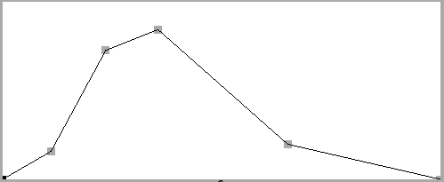
(0 0 .038 0.126 .081 0.581 .122 0.675 .224 0.158 .344 0)
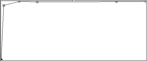
(0 95 .006 299 .043 314 .086 312 .274 313 .344 314)
by Nicky Hind
In the case of static spectra, where the amplitudes and frequencies of the various partials are constant relative to each other over time, the use of vibrato can help to `fuse' together the partials into a more unified timbre - producing a more convincing and natural sound. Essentially vibrato is an oscillation in frequency around some central perceived pitch, generally of the order of about 5 or 6Hz, and with an amplitude of around 1% of the amplitude of the basic signal. Simple sinusoidal vibrato (or any kind of periodic vibrato) on its own is far too predictable to produce a convincing result (tends to sound like some `cheesy' electric organ), so normally, a combination of periodic (sinusoidal) vibrato, and random vibrato are employed.
Here is a modified version of the instrument from `Example 1' (of part 1 of Additive Synthesis with CLM) with vibrato added. Notice firstly what structures are set up in the initialization list in order to provide vibrato, and secondly, how they are called in the Run loop. Here, a traingle-wave (rather than a sine-wave) is used for the periodic vibrato, as this is thought to model more closely the action of vibrato -- particularly in relation to bowed srting instruments.
(definstrument add-synth-vib (start-time duration frequency amplitude
			      &key
			      (partial1 1.0) (amp1 0.3) (phase1 0)
			      (partial2 2.0) (amp2 0.3) (phase2 0)
			      (partial3 3.0) (amp3 0.3) (phase3 0)
			      (amp-func1 '(0 0  50 1  100 0))
			      (amp-func2 '(0 0  50 1  100 0))
			      (amp-func3 '(0 0  50 1  100 0))
			      ;; these user variables are added for optional
			      ;; vibrato control
			      (vibrato-amplitude 0.005)
			      (vibrato-speed 5.0))

  (let* ((beg (floor (* start-time sampling-rate)))
	 (end (+ beg (floor (* duration sampling-rate))))
	 (sine1 (make-oscil :frequency (* partial1 frequency)
			    :initial-phase phase1))
	 (sine2 (make-oscil :frequency (* partial2 frequency)
			    :initial-phase phase2))
	 (sine3 (make-oscil :frequency (* partial3 frequency)
			    :initial-phase phase3))
	 (amp-env1 (make-env :envelope amp-func1
			     :scaler (* amplitude amp1)
			     :start-time start-time
			     :duration duration))
	 (amp-env2 (make-env :envelope amp-func2
			     :scaler (* amplitude amp2)
			     :start-time start-time
			     :duration duration))
	 (amp-env3 (make-env :envelope amp-func3
			     :scaler (* amplitude amp3)
			     :start-time start-time
			     :duration duration))
	 ;; Since here, vibrato is essentially implemented
	 ;; as frequency modulation, we need to get its amplitude as
	 ;; a proportion of the main frequency, and in this case,
	 ;; it must come not in terms not of Hz,
	 ;; but in radians per second (with respect
	 ;; to the sampling rate). [If this `don't make no sense'
	 ;; don't worry! we'll get to it next week when we cover
	 ;; FM for real.] First we find the main frequency
	 ;; in radians per second, this value being subsequently
	 ;; multiplied by the amplitude of the vibrato.
	 (freq-in-radians-per-sec (in-Hz frequency))
	 ;; periodic vibrato structure, feeding in the the user arguments
	 ;; defined above
	 (per-vib (make-triangle-wave :frequency vibrato-speed
				      :amplitude (* vibrato-amplitude freq-in-radians-per-sec)))
	 ;; same thing for random vibrato structure.
	 ;; ['randi' produces a series of random numbers between
	 ;; plus and minus the ampitude value, and at the rate of
	 ;; the frequency value.]
	 (ran-vib (make-randi :frequency (+ vibrato-speed 1.0)
			      :amplitude (* vibrato-amplitude freq-in-radians-per-sec))))

    (Run
     (loop for i from beg to end do
	   ;; since each oscillator is going to share the same vibrato
	   ;; value, first sum the periodic and random vibrato signals
	   ;; and collect them into the variable, 'vibrato-value'.
	   (let ((vibrato-value (+ (triangle-wave per-vib)
				   (randi ran-vib))))
	     ;; observe that 'vibrato value' becomes the second argument
	     ;; to the oscillator-activating function, 'oscil'.
	     (outa i (+	(* (env amp-env1) (oscil sine1 vibrato-value))
			(* (env amp-env2) (oscil sine2 vibrato-value))
			(* (env amp-env3) (oscil sine3 vibrato-value)))))))))
|
1. Firstly, for the sake of comparison, the sound with no vibrato -- ie. setting the vibrato amplitude to 0:
(with-sound () (add-synth-vib 0 2 220 0.5 :vibrato-amplitude 0.0))
2. Now with the default vibrato settings:
(with-sound () (add-synth-vib 0 2 220 0.5))
3. Increasing the vibrato amplitude by a factor of 10 for a more extreme result:
(with-sound () (add-synth-vib 0 2 220 0.5 :vibrato-amplitude 0.05))
Additive synthesis provides us with the capability of controlling the precise frequency -- as well as the amplitude -- of all the partials over time. This enables us to `resynthesize' spectral data (eg. from a Fourier analysis), producing results which can bear an uncanny resemblence to the original. Of course, the resynthesis process does not have to follow exactly the analysed data, and modifications can easily be made to produce unusual, but no less complex, sounds.
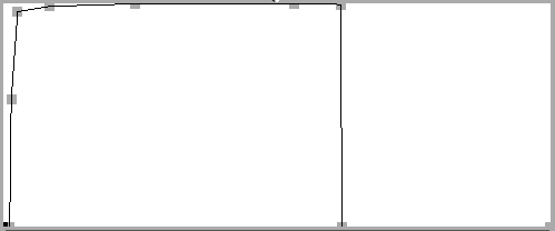
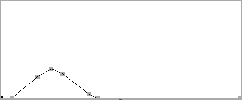
The following diagrams illustrate the difference between amplitude and frequency envelopes. For each of several partials of analysed data from a cello tone, the amplitude and frequency envelopes are shown, along with the list of break-points to which they correspond.
| 1st partial: amplitude envelope | 1st partial: frequency envelope |
 |
 |
| break-point list: (0 0 .038 0.126 .081 0.581 .122 0.675 .224 0.158 .344 0) |
break-point list: (0 95 .006 299 .043 314 .086 312 .274 313 .344 314) |
| 3rd partial: amplitude envelope | 3rd partial: frequency envelope |
 |
 |
| break-point list: (0 0 .005 0 .066 .026 .083 .021 .106 .018 .127 .006 .212 0 .344 0) |
break-point list: (0 0 .004 0 .005 540 .009 915 .029 938 .083 949 .183 950 .212 946 .213 0 .344 0) |
| 5th partial: amplitude envelope | 5th partial: frequency envelope |
 |
 |
| break-point list: (0 0 .015 0 .052 .022 .072 .03 .088 .025 .126 .004 .138 0 .3440) |
break-point list: (0 0 .013 0 .015 1342 .019 1589 .023 1554 .099 1583 .133 1581 .138 1501 .140 0 .344 0) |
As can be seen from the break-point lists, the data in this case breaks with CLM convention regarding envelopes. The time values (x-axis, first of each break-point pair) are here given in seconds (rather than normalised to 100), and the frequency of the partials appears not as a ratio of the fundamental ( as we have seen so far), but in actual Hertz. Clearly, we are getting to a point where there is a considerable amount of data to manipulate in order to resynthesize the sound: for each of the 14 partials, there are 2 lists - one for the amplitude envelope, one for the frequency envelope. In order to manage this data, it is convenient to use arrays, placing each list of data inside a different element of an array. However (as the saying goes), 'no gain, no pain', and before we look at the instrument proper, it will first be necessary to digress on to the use of arrays in LISP.
This will be as simple a description as possible, so as to not get bogged down with (at this stage) unneccessary detail.
Generally, arrays are first constructed, and then their contents assigned subsequently. To construct an array in LISP, use the function MAKE-ARRAY, giving as an argument the length of the array to be contructed. In this example we make an array of length 4, and assign it to a variable called 'beatles':
	<cl>  (setf beatles (make-array 4))

	#(NIL NIL NIL NIL)
LISP faithfully prints out the fact that an array hs been made (indicated by the # sign), plus its initial contents -- in this case defaulting to 4 NILs
To set the contents of one element of an array, we use the function AREF (standing for Array REFerence), giving as the first argument, the name of the array (ie. the variable to which it is assigned), and as the second argument, the number of the element we wish to set (counting from zero). For example, if we wish to give the first element of the array, the value 'john', this is how its done:
	<cl> (setf (aref beatles 0) 'john)

	JOHN
now examing the contents again by calling the variable-name of the array:
	<cl>  beatles

	#(JOHN NIL NIL NIL)
similarly, we can set the values for the other three elements:
	<cl> (setf (aref beatles 1) 'paul)

	PAUL
	<cl> (setf (aref beatles 2) 'george)

	GEORGE
	<cl> (setf (aref beatles 3) 'ringo)

	RINGO
now if we call the variable beatles, to which the array is assigned:
	<cl> beatles

	#(JOHN PAUL GEORGE RINGO)
To access one particular element of an array, we use the same function AREF, but this time without containing it within a SETF expression -- we just want to read it, not to set it to some value:
	<cl> (aref beatles 1)

	PAUL

	<cl> (aref beatles 0)

	JOHN
...OK, SO MUCH FOR ARRAYS!
Several types of array are used in this instrument: arrays for the amplitude and frequency envelope data (each element containing a whole list of data); arrays for the envelope structures; and arrays for the oscillator structures. As a result, the code is quite compact -- much detail being hidden in the content of the arrays.
(definstrument complete-add (begin-time duration amplitude amp-arr frq-arr)
     (let* ((beg (floor (* begin-time sampling-rate)))
	    (end (+ beg (floor (* duration sampling-rate))))
	    ;; A variable is needed to set the size of the following arrays.
	    ;; Taking the MINimum of the two input data arrays
	    ;; (amp-arr and frq-arr) is just a precaution in case there
	    ;; is an inconsistency about the input data -- don't
	    ;; `sweat' the details about this.
	    (arr-size (min (array-dimension amp-arr 0)
			   (array-dimension frq-arr 0)))
	    ;; an array in which each element is an oscilator
	    (sinusoids (make-array arr-size :element-type 'osc))
	    ;; two arrays in which each element is an envelope
	    (amp-envs (make-array arr-size :element-type 'envelope))
	    (freq-envs (make-array arr-size :element-type 'envelope)))

       ;; this loop gathers the contents of the input data arrays into
       ;; the appropriate arguments for the oscilator and envelope structures
       (loop for i below arr-size do
	     ;; freqency is set to zero, as it is handled entirely by the FM
	     ;; argument to the oscils, which in turn takes its value from
	     ;; the output from the frequency envelopes
	     (setf (aref sinusoids i) (make-oscil :frequency 0.0))
	     (setf (aref amp-envs i)
		   (make-env :envelope (aref amp-arr i) :scaler amplitude
			     :start-time begin-time :duration duration))
	     (setf (aref freq-envs i)
		   (make-env :envelope (aref frq-arr i) :scaler (in-Hz 1.0)
			     :start-time begin-time :duration duration)))

       (Run
	(loop for i from beg to end do
	      (let ((sum 0.0))
		;; for the computation of each sample value, the output of each partial
		;; (ie. each amplitude envelope multiplied by the output from
		;; each oscil with its FM input) is summed together into 'sum', and this
		;; is in turn sent to the DAC.
		(dotimes (j arr-size)
		  (incf sum (* (env (aref amp-envs j))
			       (oscil (aref sinusoids j) (env (aref freq-envs j))))))
		(outa i sum))))))
|
The hidden detail consists of the analysis data, which for convenience has been put into a seperate file, complete-add.lisp. The file also contains the above instrument definition.
1. Since the time axis of the envelopes only extends for 0.344'', we will make this the duration, and listen to a straight resynthesis:
(with-sound () (complete-add 0 0.344 1.0 amp-env-array frq-env-array))
2. Increasing the duration gives us the effect of expansion by resynthesis. Importantly, the pitch is not effected.
(with-sound () (complete-add 0 1.0 1.0 amp-env-array frq-env-array))
3. Further increasing the duration gives us an impression of what it would be like to slow down time while listening to a cello tone! Here, by a factor of 20.
(with-sound () (complete-add 0 6.88 1.0 amp-env-array frq-env-array))