Geometric Signal Theory

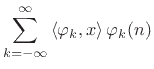
In general, signals can be expanded as a linear combination of orthonormal basis signals $\varphi_k$ [264]. In the discrete-time case, this can be expressed as

$$x(n) = \sum_{k=-\infty}^{\infty}\left<\varphi_k ,x\right> \varphi_k (n) \protect$$ (12.104)

$$n\in(-\infty,\infty), \quad x(n), \varphi_k (n) \in {\cal C}$$

where the coefficient of projection of $x$ onto $\varphi_k$ is given by

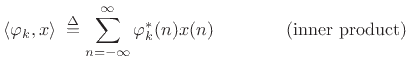$$\left<\varphi_k ,x\right> \; \isdef \sum_{n=-\infty}^{\infty}\varphi_k ^\ast(n) x(n) \qquad \qquad \hbox{(inner product)}$$ (12.105)

and the basis signals are orthonormal:

$$\left<\varphi_k ,\varphi_l \right> \eqsp \delta(k-l) \eqsp \left\{\begin{array}{ll} 1, & k=l \\ 0, & k\neq l \\ \end{array} \right. \qquad \hbox{(orthonormal)}$$ (12.106)

The signal expansion (11.104) can be interpreted geometrically as a sum of orthogonal projections of $x$ onto $\{\varphi_k \}$ , as illustrated for 2D in Fig.11.30.

Figure 11.30: Orthogonal projection in 2D.

A set of signals $\{h_k,f_k\}_{k=1}^N$ is said to be a biorthogonal basis set if any signal $x$ can be represented as

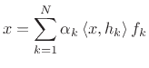$$x = \sum_{k=1}^N \alpha_k\left<x,h_k\right>f_k$$ (12.107)

where $\alpha_k$ is some normalizing scalar dependent only on $h_k$ and/or $f_k$ . Thus, in a biorthogonal system, we project onto the signals $h_k$ and resynthesize in terms of the basis $f_k$ .

The following examples illustrate the Hilbert space point of view for various familiar cases of the Fourier transform and STFT. A more detailed introduction appears in Book I [264].