Comparing (38) and (42) shows that the elements of the
normalized scattering matrix
![]() in (42) are
in (42) are
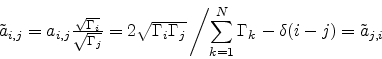 |
(59) |
 for
for
An elementary eigenvector analysis can be conducted using physical
analogies. It is well known that a symmetric matrix has orthogonal
eigenvectors. For the equal-impedance case, one eigenvector is always
![$e_0={\left[ \begin{array}{rrrr} 1 & 1 & \dots & 1\end{array} \right]}^T$](img307.png) by symmetry: this corresponds to a collision of equal pressure waves at
the junction, so the return scatter must be identical. This
corresponds to the eigenvalue 1. For the -1 eigenvalues, a
similar interpretation can be found: inject a unit pressure wave at
all the branches but one, and ``pull out'' a pressure wave having
magnitude
by symmetry: this corresponds to a collision of equal pressure waves at
the junction, so the return scatter must be identical. This
corresponds to the eigenvalue 1. For the -1 eigenvalues, a
similar interpretation can be found: inject a unit pressure wave at
all the branches but one, and ``pull out'' a pressure wave having
magnitude ![]() at the remaining branch. In this case, the return
scatter is inverted, since we have arranged that the pressure be
zero at the junction and hence at each branch termination. In this
way we can find
at the remaining branch. In this case, the return
scatter is inverted, since we have arranged that the pressure be
zero at the junction and hence at each branch termination. In this
way we can find ![]() eigenvectors analogous with
eigenvectors analogous with
![$e_1={\left[
\begin{array}{rrrr} -(N-1) & 1 & \dots & 1\end{array} \right]}^T$](img309.png) which
span the (
which
span the (![]() )-dimensional subspace associated with the
eigenvalue -1. Note that
)-dimensional subspace associated with the
eigenvalue -1. Note that ![]() is orthogonal to this subspace,
while the
is orthogonal to this subspace,
while the ![]() are not mutually orthogonal for
are not mutually orthogonal for ![]() .
.
For unequal impedances, a similar physical interpretation can be found
for the eigenvectors. If we supply equal pressure waves to all
branches at the junction, the reflected waves must be equal by symmetry, since
![]() , where
, where ![]() is the junction pressure and all the
is the junction pressure and all the
![]() are equal. Hence,
remains an eigenvector corresponding to the eigenvalue 1.
On the other hand, if we inject a unit pressure wave into all the
branches but the
are equal. Hence,
remains an eigenvector corresponding to the eigenvalue 1.
On the other hand, if we inject a unit pressure wave into all the
branches but the ![]() th and ``pull out'' a pressure wave having magnitude
th and ``pull out'' a pressure wave having magnitude
![]() at the
at the ![]() th branch, then the
junction pressure
th branch, then the
junction pressure ![]() is again forced to zero by construction and
the return scatter at any branch is the negative of the incoming
wave on that branch. In this way we can find
is again forced to zero by construction and
the return scatter at any branch is the negative of the incoming
wave on that branch. In this way we can find ![]() eigenvectors analogous with
eigenvectors analogous with
![$e_j= {\left[
\begin{array}{rrrrrrr} 1 & \dots & 1 & -{\sum_{i \neq j} \Gamma _i}/\Gamma_j & 1 & \dots &
1\end{array} \right]}^T$](img317.png) spanning the (
spanning the (![]() )-dimensional subspace
associated with the eigenvalue -1. In this case, none of the eigenvectors
is necessarily orthogonal to the others.
)-dimensional subspace
associated with the eigenvalue -1. In this case, none of the eigenvectors
is necessarily orthogonal to the others.
The foregoing is an example of how physical intuition can help in finding algebraic properties of a given matrix in physical applications.
Another property of the scattering matrix
![]() is that it is its
own inverse:
is that it is its
own inverse:
![]() . This corresponds physically to the fact
that if the results of a scattering operation are fed back to the same
junction as incoming waves, the result must be the inverse of the
original scattering. An implication of this is that lossless
scattering networks can be run in reverse, i.e., by changing the
directions of all the delay lines and computing the junctions as
dictated by the wave impedances, the network will compute its own
inverse. If there are inputs and outputs, they must be interchanged.
. This corresponds physically to the fact
that if the results of a scattering operation are fed back to the same
junction as incoming waves, the result must be the inverse of the
original scattering. An implication of this is that lossless
scattering networks can be run in reverse, i.e., by changing the
directions of all the delay lines and computing the junctions as
dictated by the wave impedances, the network will compute its own
inverse. If there are inputs and outputs, they must be interchanged.