Next |
Prev |
Up |
Top
|
Index |
JOS Index |
JOS Pubs |
JOS Home |
Search
The Fourier transform of a complex Gaussian pulse is derived in
§D.8 of Appendix D:
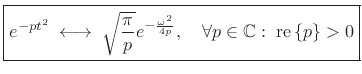 |
(11.27) |
This result is valid when  is complex.
Writing
in terms of real variables
is complex.
Writing
in terms of real variables
 and
and  as
as
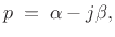 |
(11.28) |
we have
![$\displaystyle x(t) \eqsp e^{-p t^2} \eqsp e^{-\alpha t^2} e^{j\beta t^2} \eqsp e^{-\alpha t^2} \left[\cos(\beta t^2) + j\sin(\beta t^2)\right].$](img1868.png) |
(11.29) |
That is, for
complex,  is a chirplet (Gaussian-windowed
chirp). We see that the chirp oscillation frequency is zero at time
is a chirplet (Gaussian-windowed
chirp). We see that the chirp oscillation frequency is zero at time
 . Therefore, for signal modeling applications, we typically add
in an arbitrary frequency offset at time 0, as described in the next
section.
. Therefore, for signal modeling applications, we typically add
in an arbitrary frequency offset at time 0, as described in the next
section.
Next |
Prev |
Up |
Top
|
Index |
JOS Index |
JOS Pubs |
JOS Home |
Search
[How to cite this work] [Order a printed hardcopy] [Comment on this page via email]