Digital waveguide techniques have been used to develop efficient physical models of musical instruments since the early 1990s [SmithSmith1987,Smith IIISmith III2003,Van Duyne and SmithVan Duyne and Smith1993a,Van Duyne and SmithVan Duyne and Smith1993b]. The digital waveguide model can be used to reduce the computational cost of physical models based on numerical integration of the wave equation by three orders of magnitude by simulating the traveling waves with digital delay lines.
The one-dimensional digital waveguide can be extended into a two-dimensional digital waveguide mesh [Van Duyne and SmithVan Duyne and Smith1993a,Van Duyne and SmithVan Duyne and Smith1993b]. The structure of the 2-D digital waveguide mesh can be viewed as a layer of parallel vertical waveguides superimposed on a layer of parallel horizontal waveguides intersecting each other at 4-port scattering junctions as shown in Figure 2.
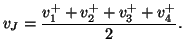
In a lossless case, the scattering junction has two physical
constraints: 1) the velocities of all the strings at the junction must
be equal, i.e.,
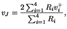
Combining the two series junction constraints with the wave impedance
relations between force and velocity wave variables defined as ![]() and
and ![]() , and with the wave variable definitions,
, and with the wave variable definitions,
![]() , and
, and
![]() , we can derive the
lossless scattering equations for the junctions in which four strings
intersect,
, we can derive the
lossless scattering equations for the junctions in which four strings
intersect,