The first step is to make a second-order digital filter with zero
damping by abutting two unit-sample sections of waveguide medium, and
terminating on the left and right with perfect reflections, as shown
in Fig.1. The wave impedance in section ![]() is given by
is given by
![]() , where
, where ![]() is air density,
is air density, ![]() is the
cross-sectional area of tube section
is the
cross-sectional area of tube section ![]() , and
, and ![]() is sound speed. The
reflection coefficient is determined by the impedance discontinuity
via
is sound speed. The
reflection coefficient is determined by the impedance discontinuity
via
![]() . It turns out that to obtain sinusoidal
oscillation, one of the terminations must provide an inverting
reflection while the other is non-inverting.
. It turns out that to obtain sinusoidal
oscillation, one of the terminations must provide an inverting
reflection while the other is non-inverting.
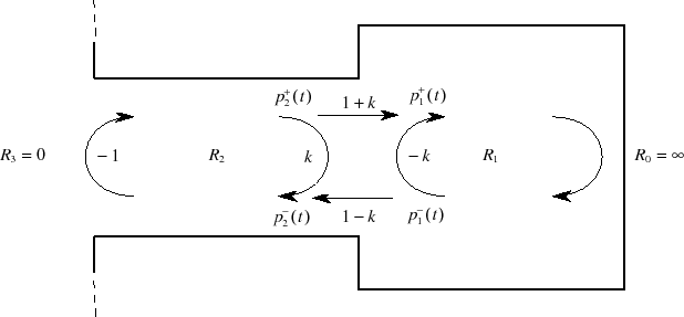 |
At the junction between sections ![]() and
and ![]() , the signal is partially
transmitted and partially reflected such that energy is conserved,
i.e., we have lossless scattering. The formula for the
reflection coefficient
, the signal is partially
transmitted and partially reflected such that energy is conserved,
i.e., we have lossless scattering. The formula for the
reflection coefficient ![]() can be derived from the physical
constraints that (1) pressure is continuous across the junction, and
(2) there is no net flow into or out of the junction. For traveling
pressure waves
can be derived from the physical
constraints that (1) pressure is continuous across the junction, and
(2) there is no net flow into or out of the junction. For traveling
pressure waves ![]() and volume-velocity waves
and volume-velocity waves ![]() , we
have
, we
have
![]() and
and
![]() . The physical
pressure and volume velocity are obtained by summing the
traveling-wave components.
. The physical
pressure and volume velocity are obtained by summing the
traveling-wave components.
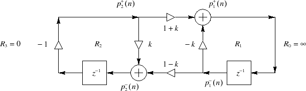
The discrete-time simulation for the physical system of Fig.1 is shown in Fig.2. The propagation time from the junction to a reflecting termination and back is one sample period. The half sample delay from the junction to the reflecting termination has been commuted with the termination and combined with the half sample delay to the termination. This is a special case of a ``half-rate'' waveguide filter [6].
Since only two samples of delay are present, the digital system is at
most second order, and since the coefficients are real, at most one
frequency of oscillation is possible in ![]() .
.
The scattering junction shown in the figure is called the Kelly-Lochbaum junction in the literature on lattice and ladder digital filters [2]. While it is the most natural from a physical point of view, it requires four multiplies and two additions for its implementation.
It is well known that lossless scattering junctions can be implemented
in a variety of equivalent forms, such as the two-multiply and even
one-multiply junctions. However, most have the disadvantage of not
being normalized in the sense that changing the reflection
coefficient ![]() changes the amplitude of oscillation. This can be
understood physically by noting that a change in
changes the amplitude of oscillation. This can be
understood physically by noting that a change in ![]() implies a
change in
implies a
change in ![]() . Since the signal power contained in a waveguide
variable, say
. Since the signal power contained in a waveguide
variable, say ![]() , is
, is
![$\left[p_1^+(n)\right]^2/R_1$](img37.png) , we find that modulating the
reflection coefficient corresponds to modulating the signal energy
represented by the signal sample in at least one of the two delay
elements. Since energy is proportional to amplitude squared, energy
modulation implies amplitude modulation.
, we find that modulating the
reflection coefficient corresponds to modulating the signal energy
represented by the signal sample in at least one of the two delay
elements. Since energy is proportional to amplitude squared, energy
modulation implies amplitude modulation.
The well-known normalization procedure is to replace the traveling
pressure waves ![]() by ``root-power'' pressure waves
by ``root-power'' pressure waves
![]() so that signal power is just the square of a signal
sample
so that signal power is just the square of a signal
sample
![]() . When this is done, the scattering junction
transforms from the Kelly-Lochbaum or one-multiply form into the
normalized ladder junction in which the reflection coefficients
are again
. When this is done, the scattering junction
transforms from the Kelly-Lochbaum or one-multiply form into the
normalized ladder junction in which the reflection coefficients
are again ![]() , but the forward and reverse transmission
coefficients become
, but the forward and reverse transmission
coefficients become ![]() . Defining
. Defining
![]() , the
transmission coefficients can be seen as
, the
transmission coefficients can be seen as ![]() , and we arrive
essentially at the coupled form, or two-dimensional vector
rotation considered in [1].
, and we arrive
essentially at the coupled form, or two-dimensional vector
rotation considered in [1].
An alternative normalization technique is based on the digital
waveguide transformer [6]. The purpose of a
``transformer'' is to ``step'' the force variable (pressure in our
example) by some factor ![]() without scattering and without affecting
signal energy. Since traveling signal power is proportional to
pressure times velocity
without scattering and without affecting
signal energy. Since traveling signal power is proportional to
pressure times velocity ![]() , it follows that velocity must be
stepped by the inverse factor
, it follows that velocity must be
stepped by the inverse factor ![]() to keep power constant. This is
the familiar behavior of transformers for analog electrical circuits:
voltage is stepped up by the ``turns ratio'' and current is stepped
down by the reciprocal factor. Now, since
to keep power constant. This is
the familiar behavior of transformers for analog electrical circuits:
voltage is stepped up by the ``turns ratio'' and current is stepped
down by the reciprocal factor. Now, since ![]() , traveling
signal power is equal to
, traveling
signal power is equal to
![]() . Therefore, stepping
up pressure through a transformer by the factor
. Therefore, stepping
up pressure through a transformer by the factor ![]() corresponds to
stepping up the wave impedance
corresponds to
stepping up the wave impedance ![]() by the factor
by the factor ![]() . In other
words, the transformer raises pressure and decreases volume velocity
by raising the wave impedance (narrowing the acoustic tube) like a
converging cone.
. In other
words, the transformer raises pressure and decreases volume velocity
by raising the wave impedance (narrowing the acoustic tube) like a
converging cone.
If a transformer is inserted in a waveguide immediately to the left,
say, of a scattering junction, it can be used to modulate the the wave
impedance ``seen'' to the left by the junction without having to use
root-power waves in the simulation. As a result, the one-multiply
junction can be used for the scattering junction, since the junction
itself is not normalized. Since the transformer requires two
multiplies, a total of three multiplies can effectively implement a
normalized junction, where four were needed before. Finally, in just
this special case, one of the transformer coefficients can be commuted
with the delay element on the left and combined with the other
transformer coefficient. For convenience, the ![]() coefficient on the
left is commuted into the junction so it merely toggles the signs of
inputs to existing summers. These transformations lead to the final
form shown in Fig.3.
coefficient on the
left is commuted into the junction so it merely toggles the signs of
inputs to existing summers. These transformations lead to the final
form shown in Fig.3.
The ``tuning coefficient'' is given by
![]() , where
, where
![]() is the desired oscillation frequency in Hz at sample
is the desired oscillation frequency in Hz at sample ![]() , and
, and
![]() is the sampling period in seconds. The ``amplitude coefficient''
is
is the sampling period in seconds. The ``amplitude coefficient''
is
![]() , where
, where
![]() is the
exponential growth or decay per sample (
is the
exponential growth or decay per sample (![]() for constant
amplitude), and
for constant
amplitude), and ![]() is the normalizing transformer ``turns ratio''
given by
is the normalizing transformer ``turns ratio''
given by
![]() . When both amplitude and
frequency are constant, we have
. When both amplitude and
frequency are constant, we have ![]() , and only the tuning
multiply is operational. When frequency changes, the amplitude
coefficient deviates from unity for only one time sample to normalize
the oscillation amplitude.
, and only the tuning
multiply is operational. When frequency changes, the amplitude
coefficient deviates from unity for only one time sample to normalize
the oscillation amplitude.
When amplitude and frequency are constant, there is no gradual exponential
growth or decay due to round-off error. This happens because the only
rounding is at the output of the tuning multiply, and all other
computations are exact. Therefore, quantization in the tuning coefficient
can only cause quantization in the frequency of oscillation. Note that any
one-multiply digital oscillator should have this property. In contrast,
the only other known normalized oscillator, the coupled form, does
exhibit exponential amplitude drift because it has two coefficients
![]() and
and
![]() which, after quantization, no longer
obey
which, after quantization, no longer
obey ![]() for most tunings.
for most tunings.