| (2.7) |
An approximate discrete-time numerical solution of Eq.(1.6) is provided by
Let
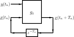
![$\displaystyle g_{t_n}[\underline{x}(t_n),\underline{u}(t_n)] \isdefs \underline{x}(t_n) + T_n\,f_{t_n}[\underline{x}(t_n),\underline{u}(t_n)].
$](img217.png)
Then we can diagram the time-update as in Fig.1.7. In this form, it is clear that
This is a simple example of numerical integration for solving
an ODE, where in this case the ODE is given by Eq.(1.6) (a very
general, potentially nonlinear, vector ODE). Note that the initial
state
![]() is required to start Eq.(1.7) at time zero;
the initial state thus provides boundary conditions for the ODE at
time zero. The time sampling interval
is required to start Eq.(1.7) at time zero;
the initial state thus provides boundary conditions for the ODE at
time zero. The time sampling interval ![]() may be fixed for all
time as
may be fixed for all
time as ![]() (as it normally is in linear, time-invariant
digital signal processing systems), or it may vary adaptively
according to how fast the system is changing (as is often needed for
nonlinear and/or time-varying systems). Further discussion of
nonlinear ODE solvers is taken up in §7.4, but for most of
this book, linear, time-invariant systems will be emphasized.
(as it normally is in linear, time-invariant
digital signal processing systems), or it may vary adaptively
according to how fast the system is changing (as is often needed for
nonlinear and/or time-varying systems). Further discussion of
nonlinear ODE solvers is taken up in §7.4, but for most of
this book, linear, time-invariant systems will be emphasized.
Note that for handling switching states (such as op-amp comparators and the like), the discrete-time state-space formulation of Eq.(1.7) is more conveniently applicable than the continuous-time formulation in Eq.(1.6).