Next |
Prev |
Up |
Top
|
Index |
JOS Index |
JOS Pubs |
JOS Home |
Search
For two of the schemes that we will examine (hexagonal and tetrahedral), it will be necessary to analyze a vectorized system of difference equations. In general, the analysis of vector forms is considerably more difficult; the typical approach will invoke the Kreiss Matrix Theorem [8], which is a set of equivalent conditions which can be used to check the boundedness of a particular amplification matrix. In the general vector case we will be analyzing the evolution of a  -element vector
![$ \hat{{\bf U}}_{\mbox{{\scriptsize\boldmath $\beta$}}}(n) = [\hat{U}_{1,\mbox{{...
...\beta$}}}(n), \hdots, \hat{U}_{q,\mbox{{\scriptsize\boldmath $\beta$}}}(n)]^{T}$](img76.png) of spatially Fourier-transformed functions of
of spatially Fourier-transformed functions of
 . The
. The  norm is defined by
where  denotes transpose conjugation.
The schemes for the wave equation that we will examine, however, have a relatively simple form. The column vector of grid spatial frequency spectra
 satisfies an equation of the form
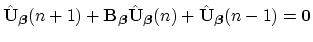 |
(11) |
for some Hermitian matrix function of
,
 . Because
is Hermitian, we may write
. Because
is Hermitian, we may write
 , for some unitary matrix
 , and a real diagonal matrix

 containing the eigenvalues of
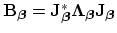
. As such, we may change variables via
containing the eigenvalues of
. As such, we may change variables via
 , to get
 |
(12) |
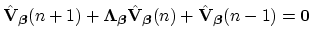
The system thus decouples into a system of scalar two-step spectral update equations; because
and
 are related by a unitary transformation, we have
 , and we may apply stability tests to the uncoupled system (11). We thus require that the eigenvalues of
, namely
, and we may apply stability tests to the uncoupled system (11). We thus require that the eigenvalues of
, namely
 for
for
 , which are the elements on the diagonal of
, all satisfy
, which are the elements on the diagonal of
, all satisfy
 |
(13) |
At frequencies
 for which any of the eigenvalues satisfies (12) with equality, then we may again have the same problem with mild linear growth in the solution.
Next |
Prev |
Up |
Top
|
Index |
JOS Index |
JOS Pubs |
JOS Home |
Search
Download vonn.pdf
