Next  |  Prev  |  Up  |  Top  |  Index  |  JOS Index  |  JOS Pubs  |  JOS Home  |  Search


FDA of the Ideal String

Substituting the FDA into the wave equation gives

$\displaystyle K\frac{y(t,x+X) - 2 y(t,x) + y(t,x-X)}{X^2} =
\epsilon \frac{y(t+T,x) - 2 y(t,x) + y(t-T,x)}{T^2}
$

which can be solved to yield the following recursion for the string displacement:
$\displaystyle y(t+T,x)$ $\displaystyle =$ $\displaystyle \frac{KT^2}{\epsilon X^2}
\left[ y(t,x+X) - 2 y(t,x) + y(t,x-X)\right]$  
    $\displaystyle \qquad\qquad\qquad\qquad + 2 y(t,x) - y(t-T,x)$  

In a practical implementation, it is common to set $ T=1,\,
X=(\sqrt{K/\epsilon })T$, and evaluate on the integers $ t=nT=n$ and $ x=mX=m$ to obtain the difference equation

$\displaystyle y(n+1,m) = y(n,m+1) + y(n,m-1) - y(n-1,m)$ (G.6)

Thus, to update the sampled string displacement, past values are needed for each point along the string at time instants $ n$ and $ n-1$. Then the above recursion can be carried out for time $ n+1$ by iterating over all $ m$ along the string.

Perhaps surprisingly, it is shown in Appendix M that the above recursion is exact at the sample points in spite of the apparent crudeness of the finite difference approximation [420]. The FDA approach to numerical simulation was used by Pierre Ruiz in his work on vibrating strings [365], and it is still in use today [71,72].

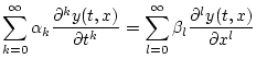
When more terms are added to the wave equation, corresponding to complex losses and dispersion characteristics, more terms of the form $ y(n-l,m-k)$ 
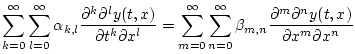
appear in (G.6). These higher-order terms correspond to frequency-dependent losses and/or dispersion characteristics in the FDA. All linear differential equations with constant coefficients give rise to some linear, time-invariant discrete-time system via the FDA. A general subclass of the linear, time-invariant case giving rise to ``filtered waveguides'' is

$\displaystyle \sum_{k=0}^\infty \alpha_k \frac{\partial^k y(t,x)}{\partial t^k} = \sum_{l=0}^\infty \beta_l \frac{\partial^l y(t,x)}{\partial x^l}$ (G.7)

while the fully general linear, time-invariant 2D case is

$\displaystyle \sum_{k=0}^\infty \sum_{l=0}^\infty \alpha_{k,l} \frac{\partial^k...
...infty \beta_{m,n} \frac{\partial^m\partial^n y(t,x)}{\partial x^m \partial x^n}$ (G.8)

A nonlinear example is

$\displaystyle \frac{\partial y(t,x)}{\partial t} = \left(\frac{\partial y(t,x)}{\partial x}\right)^2$ (G.9)

and a time-varying example can be given by

$\displaystyle \frac{\partial y(t,x)}{\partial t} = t^2\frac{\partial y(t,x)}{\partial x}$ (G.10)


Next  |  Prev  |  Up  |  Top  |  Index  |  JOS Index  |  JOS Pubs  |  JOS Home  |  Search

[How to cite and copy this work] 
``Physical Audio Signal Processing for Virtual Musical Instruments and Digital Audio Effects'', by Julius O. Smith III, (December 2005 Edition).
Copyright © 2006-07-01 by Julius O. Smith III
Center for Computer Research in Music and Acoustics (CCRMA),   Stanford University
CCRMA  [Automatic-links disclaimer]