Finding the Eigenstructure of A

Starting with the defining equation for an eigenvector $\underline{e}$ and its corresponding eigenvalue $\lambda$ ,

$$A\underline{e}_i= \lambda_i \underline{e}_i,\quad i=1,2$$

we get

$$\left[\begin{array}{cc} c & c-1 \\ [2pt] c+1 & c \end{array}\right] \left[\begin{array}{c} 1 \\ [2pt] \eta_i \end{array}\right] = \left[\begin{array}{c} \lambda_i \\ [2pt] \lambda_i \eta_i \end{array}\right]. \protect$$ (G.23)

We normalized the first element of $\underline{e}_i$ to 1 since $g\underline{e}_i$ is an eigenvector whenever $\underline{e}_i$ is. (If there is a missing solution because its first element happens to be zero, we can repeat the analysis normalizing the second element to 1 instead.)

Equation (G.23) gives us two equations in two unknowns:

$$c+\eta_i (c-1) = \lambda_i \protect$$ (G.24)

$$(1+c) +c\eta_i = \lambda_i \eta_i$$ (G.25)

Substituting the first into the second to eliminate $\lambda_i$ , we get

$$\begin{eqnarray*} 1+c+c\eta_i &=& [c+\eta_i (c-1)]\eta_i = c\eta_i + \eta_i ^2 (c-1)\\ \,\,\Rightarrow\,\,1+c &=& \eta_i ^2 (c-1)\\ \,\,\Rightarrow\,\,\eta_i &=& \pm \sqrt{\frac{c+1}{c-1}}. \end{eqnarray*}$$

Thus, we have found both eigenvectors

$$\begin{eqnarray*} \underline{e}_1&=&\left[\begin{array}{c} 1 \\ [2pt] \eta \end{array}\right],\qquad \underline{e}_2=\left[\begin{array}{c} 1 \\ [2pt] -\eta \end{array}\right], \quad \hbox{where}\\ \eta&\isdef &\sqrt{\frac{c+1}{c-1}}. \end{eqnarray*}$$

They are linearly independent provided $\eta\neq0\Leftrightarrow c\neq -1$ and finite provided $c\neq 1$ .

We can now use Eq.(G.24) to find the eigenvalues:

$$\lambda_i = c + \eta_i (c-1) = c \pm \sqrt{\frac{c+1}{c-1} (c-1)^2} = c \pm \sqrt{c^2-1}$$

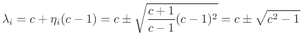
Assuming $\left\vert c\right\vert<1$ , the eigenvalues are

$$\lambda_i = c \pm j\sqrt{1-c^2} \protect$$ (G.26)

and so this is the range of $c$ corresponding to sinusoidal oscillation. For $\left\vert c\right\vert>1$ , the eigenvalues are real, corresponding to exponential growth and decay. The values $c=\pm 1$ yield a repeated root (dc or $f_s/2$ oscillation).

Let us henceforth assume $-1 < c < 1$ . In this range $\theta \isdef \arccos(c)$ is real, and we have $c=\cos(\theta)$ , $\sqrt{1-c^2} = \sin(\theta)$ . Thus, the eigenvalues can be expressed as follows:

$$\begin{eqnarray*} \lambda_1 &=& c + j\sqrt{1-c^2} = \cos(\theta) + j\sin(\theta) = e^{j\theta}\\ \lambda_2 &=& c - j\sqrt{1-c^2} = \cos(\theta) - j\sin(\theta) = e^{-j\theta}\\ \end{eqnarray*}$$

Equating $\lambda_i$ to $e^{j\omega_i T}$ , we obtain $\omega_i T = \pm \theta$ , or $\omega_i = \pm \theta/T = \pm f_s\theta = \pm f_s\arccos(c)$ , where $f_s$ denotes the sampling rate. Thus the relationship between the coefficient $c$ in the digital waveguide oscillator and the frequency of sinusoidal oscillation $\omega$ is expressed succinctly as

$$\fbox{$\displaystyle c = \cos(\omega T).$}$$

We see that the coefficient range (-1,1) corresponds to frequencies in the range $(-f_s/2,f_s/2)$ , and that's the complete set of available digital frequencies.

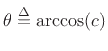
We have now shown that the system of Fig.G.3 oscillates sinusoidally at any desired digital frequency $\omega$ rad/sec by simply setting $c=\cos(\omega T)$ , where $T$ denotes the sampling interval.