Since our example transfer function
(from Eq.(3.4)) is a ratio of polynomials in
The poles and zeros for this simple example are easy to work out by hand. The zeros are located in the
where we assume
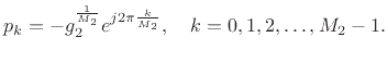
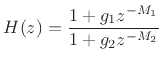
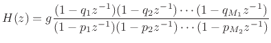
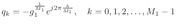
Figure 3.12 gives the pole-zero diagram of the specific example filter
![]() . There are three zeros,
marked by `O' in the figure, and five poles, marked by
`X'. Because of the simple form of digital comb filters, the
zeros (roots of
. There are three zeros,
marked by `O' in the figure, and five poles, marked by
`X'. Because of the simple form of digital comb filters, the
zeros (roots of ![]() ) are located at 0.5 times the three cube
roots of -1 (
) are located at 0.5 times the three cube
roots of -1 (
![]() ), and similarly the poles (roots
of
), and similarly the poles (roots
of ![]() ) are located at 0.9 times the five 5th roots of -1
(
) are located at 0.9 times the five 5th roots of -1
(
![]() ). (Technically, there are also two more
zeros at
). (Technically, there are also two more
zeros at ![]() .) The matlab code for producing this figure is simply
.) The matlab code for producing this figure is simply
[zeros, poles, gain] = tf2zp(B,A); % Matlab or Octave
zplane(zeros,poles); % Matlab Signal Processing Toolbox
                     % or Octave Forge
where B and A are as given in Fig.3.11.
The pole-zero plot utility zplane is
contained in the Matlab Signal Processing Toolbox, and in the
Octave Forge collection. A similar plot is produced bysys = tf2sys(B,A,1); pzmap(sys);where these functions are both in the Matlab Control Toolbox and in Octave. (Octave includes its own control-systems tool-box functions in the base Octave distribution.)
![\includegraphics[width=\twidth]{eps/epz}](img354.png)