Measuring the CryBaby Frequency Response

Measuring the frequency response of a wah pedal is relatively easy because it is a single-input, single-output, analog audio filter, with quarter-inch input/output jacks. A CryBaby pedal¹⁶ was hooked up to an input and output of a Gina3G audio interface connected to a Linux PC (Red Hat Fedora 7 distribution) with Planet CCRMA installed. The response measurements shown in Figures 14 through 16 were carried out in pd and Octave¹⁷ using software from the RealSimple Transfer Function Measurement Toolbox (RTFMT) [1].¹⁸The Octave command-line for generating the test input data (a sine sweep whose frequency increases exponentially with time) was as follows:

  generate_sinesweeps(40,10000,48000,2);

This specifies a sine sweep from 40 Hz to 10 kHz lasting 2 seconds, with the sampling rate set to 48 kHz. Next, the shell command-line

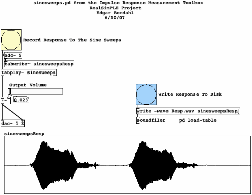
  pd sinesweeps.pd

opens the pd patch shown in Fig.17. This pd patch (also distributed with the RTFMT) plays the sinesweep and records the response when the button labeled ``Record Response To The Sine Sweeps'' is clicked. The captured sweep-response is displayed so that the ``Output Volume''can be adjusted to achieve a good level. When the level looks good, the captured response is written to Resp.wav by clicking the button labeled ``Write Response To Disk.'' This was repeated for three settings of the wah pedal as described above (min, middle, and max pedal angles).

Figure 17: sinesweeps.pd after making a measurement with an appropriate input level (from [1]).

The captured response is in the form of a measured impulse response. The next step is to convert each of the three measured impulse responses to resonator filter coefficients. There are many ways of doing this [11]. For this exercise, the matlab¹⁹ scripts shown in Figures 18 and 19 were used.

Figure: Listing of a matlab script for estimating the Q and pole-frequency in three measured frequency responses for the CryBaby wah pedal at three different pedal settings. The function invfreqsmethod is defined in Fig.19.

 

f1 = 40; f2 = 10000;   % used in filename (can't change)
f1z = 300; f2z = 3000; % zoom-in range (improves estimates)
del = [3000 2000 2000]; % measurement system delay (samples)
dur = [2048 1024 1024]; % impulse-response duration to take
dir = sprintf('wah-2sec-%dHz-%dkHz',f1,f2/1000);
Q = zeros(1,3);
wp = zeros(1,3);
for i=1:3
  ifn = sprintf('%s/wah%dImpResp.wav',dir,i-1);
  [wahir,fs] = wavread(ifn);
  if (del(i)+dur(i))>length(wahir)
    error('Signal is too short (less than system delay)'); 
  end
  wi = wahir(del(i)+1:del(i)+dur(i));
  [Qi,wpi,Hp,Hd,w] = invfreqsmethod(wi,f1z,f2z,fs);
  Q(i) = Qi; wp(i) = wpi;
  disp('PAUSING - RETURN to continue'); pause;
end
Q               % print out estimated Q values
fp = wp/(2*pi)  % print out estimated pole frequencies