Bandpass and other Filters

Before digging into filters and digital signal processing, it might be worth to stop and reflect on the object of using a machine for music generation. Are we getting too mechanical that we need mechanisms for achieving ideas and creations?. There is a tendency to think that products resulting from a system, a machine, are molded to be mass produced and widely distributed. In this way an idea turns into a 'template' and its innovative features and success translate into patterns for replication of a hit. To think about a subject matter under this framework seems too constrained and thus limiting a wide array of features encompassed under the terms of computer music.

More than three decades have passed since our first international computer music conference (ICMC). Furthermore, The Computer Music Journal (CMJ) has been publishing papers for almost half a century. ICMS's are still happening every year and CMJ still publishing state of the art, stating and not being too idealistic, facts that a computer is far from being just a machine and probing music produced with computers is not just templates of mass produced patterns. Likewise papers keep publishing and conferences still going on periodically because in part early promises of computer technology have not materialized and remain as goals to be achieved for the faithful pursuer.

Even so, a lot has been achieved, hence horizons have widened for many. Instead of a machine, a computer is more like a 'lab', an environment to test ideas, procedures, methods, and more. With it, prototyping, modeling, arranging, editing and of course, creation of works among others are attained. Given this scope, a composer can question aesthetic issues, musical possibilities within a broad spectrum of past-present and future. Beyond analysis and synthesis techniques people can go further into frameworks encompassing new definitions of performance, interactions, listening spaces, just to name a few.

If music is a tradition, the use of a computer follows experiments and language searches on the real of the second half of the twentieth century not leaving ideas of the first half and even before. Recall “Sound Houses” in the “New Atlantis” hinted by Sir Francis Bacon (circa 1627):

“ We have also sound-houses, where we practice and demonstrate all sounds and their generation. We have harmonies, which you have not, of quarter-sounds and lesser slides of sounds. Divers instruments of music likewise to you unknown, some sweeter than any you have, together with bells and rings that are dainty and sweet...”

It does not look computer music is coerced to “digital media” as some want to label it. It goes further beyond those bounds. An advantage of the LAB analogy expressed before, is that ideas on other domains of knowledge can be tested and confronted to the music domain by means of an algorithm. For instance the idea of digital filtering came from replicating a physical mechanism into a discrete computer model of its functionality. Namely, tape recorders of the fifties and sixties. On the issue of “Composers and the Computer” Curtis Roads (circa 1985) abetted hints for what computer techniques beyond a machine might certainly course people pursuing this practice:

Some digital techniques are little more than precise versions of previous mechanical or analog processes. But precision is not the most important attribute of the computer. What the computer offers the composer is programmability. -The extension of functionality in any direction-...

... The computer can be used to control a synthesizer, to process sounds, to edit scores, to create scores according to composer-specified rules, to print music, to analyze music, and to act as a partner in improvisation.

Signal processing on a digital domain in a computer is an opportunity for ingenuity. Thereby, it is a method for testing ideas and for discoveries. Though, it can be challenging, it is usually rewarding. Filters process media and when in audio domains they become hammer and chisel for crafting sound in music works. A filter can remove, reduce or even strengthen certain bands of frequencies in a signal. There are infinite impulse response filters (IIR) and finite impulse response filters (FIR). On IIR filters output is recirculated into input in such a way that sound could keep recirculating in a loop forever, depending upon settings of the feedback volume control. Therefore, infinite repeats translate into infinite response. On FIR filters repeats are finite. Important to note here that 'repeats' mean 'delays' on DSP parlance. The frequency response of a filter shows which frequencies a filter passes and which it rejects. Filters are classified by the kind of frequencies they pass as follows:

• Lowpass: Low frequencies are allowed to pass through.
• Highpass: High frequencies are allowed to pass through.
• Bandpass: A band of frequencies between a lower and upper limit are allowed to pass through.
• Bandreject: A band of frequencies between a lower and upper limit are blocked.
• Allspass: All frequencies are allowed to pass equally. this kind of filter changes only the phase of the signal.

More complex filters can be made out of combinations of these simpler filters. Likewise, any complex filter can be broken down into combinations of above filters. In addition to modifying the amplitude of signals based on their frequency, filters commonly modify the phase of the signals, delaying phases of some frequencies more than others. We start our examples by trying out a band pass on Snd. Here we want to get a band of frequencies in-between lower and upper frequencies. In other words we want to isolate some frequencies given a center frequency and a bandwidth. There are several ways to design a Bandpass but here and for the purpose of getting your hands right into DSP Bandpass from a FIR filter design is going to be tried.

Snd's s7 is a full featured DSP environment stocking plenty of tools to do almost any kind of conceivable signal processing techniques. You can have a canonical filter of any order and type in addition to IIR and FIR filters of any order. You just need to supply filter coefficients accordingly into the filter's generator. It is not fair to think that DSP is just boiling down recipes for getting right coefficients for a given application. Nevertheless for the time being, it is worth thinking about coefficients for our filtering applications. For the implementation of a Bandpass we need to find “the recipe” for finding its coefficients. To understand this procedure it is helpful to understand the workings of an FIR filter.

Recall that a finite impulse response FIR filter is a filter whose impulse response (or response to any finite length input) is of finite duration, because it settles to zero in finite time. An impulse response might be thought of as a single '1' (one) followed by many '0' (zeroes), on the digital discrete domain. Zeroes will come out after the one has made its way through the delay line of the filter. Most digital filters are function of a delay line. A discrete-time FIR filter of order N, each value of the output sequence is a weighted sum of the most recent input values:

$$y_n = b_0x_n+b_1x_{n-1}+ \ldots + b_Nx_{n-N}$$

$$= \sum_{i=0}^N b_ix_{n-i},$$

Where, 'x[n]' is the input signal, 'y[n]' is the output signal, 'N' is the filter order; 'b_i' is the value of the impulse response at the i'th sample for 0 ≤ i ≤ N. Values of 'b' might also be referred as filter coefficients.

For an analytical explanation of FIR filters or for further information “HERE” or, go to Julius Smith's General Filters page: “HERE”

Several Bandpass implementations can be found on “dsp.scm”. Below is Bill Shotstaedt's code for a Bandpass FIR filter structure of order 30. While defining FIRs within Snd's filter generator, order and xcoeffs need to be supplied. The “order” argument should be one greater than the nominal filter order. “xcoeffs” are all coefficients in an array or a vector of size “order”.

 		 
(define* (make-bandpass flo fhi (len 30))
  (let ((arrlen (+ 1 (* 2 len))))
    (do ((arr (make-float-vector arrlen))
	 (i (- len) (+ i 1)))
	((= i len)
	 (make-fir-filter arrlen arr))     
      (let ((k (+ i len))
	    (denom (* pi i))
	    (num (- (sin (* fhi i)) (sin (* flo i)))))
	(set! (arr k)
	      (if (= i 0)
		  (/ (- fhi flo) pi)
		  (* (/ num denom) 
		     (+ .54 (* .46 (cos (/ (* i pi) len)))))))))
    ))

 		 
(define bandpass fir-filter)

Following are equations for calculating coefficients for this filter and where W_0 is lower frequency and W_1 is upper frequency. N is the order of the the filter and n is each coefficient number. Keep on mind that most filter definitions wor with radian frequencies. If Hertz are easier to handle then frequencies need to be converted.

$$b_0=\frac{\omega_1-\omega_0}{\pi}$$

$$b_n=\frac{\sin(\omega_1n) - \sin(\omega_0n)}{\pi n} \cos(\frac{\pi n}{N})$$

Each value is stored in an array so that we have a vector with all coefficients to be pass into the filter unit generator of Snd.. Below there is a function definition to see if the filter really works.

 		 

(define* (bpass-noise start dur amp cfq bwf 
			 (len 30))
  (let* ((beg (seconds->samples start))
	 (q (hz->radians cfq))                        ;; center 'cut' frequency to radians
	 (bw (hz->radians bwf))                       ;; bandwidth frequency to radians
	 (loc (- q (/ bw 2)))                         ;; lower frequency bound
	 (hic (+ q (/ bw 2)))                         ;; upper frequency bound
	 (b0 (make-bandpass loc hic len))             ;; make bandpass structure
 	 (ra (make-rand :frequency sampling-rate 
			:amplitude (* 2 amp)))        ;; create random noise generator
	 (end (+ beg (seconds->samples dur))))
    ;;
    (do ((i beg (+ i 1)))
	((= i end))
      (outa i (bandpass b0 (rand ra)))
      ) ))

Copy-and-paste -all-of-the-above- code into a new file and save it as “bandpass.cms”.

• Load “bandpass.cms”into Snd:

  
           (load "bandpass.cms")        
  
  
  

• Now we can try function calls to listen the effect of this bandpass on a noise source. On our function definition “bpass-noise” last couple of arguments are center frequency and bandwidth. On this case we have a center frequency of 3000 Hz. and a bandwidth of 1000 Hz. For this call we are using default filter order of 30. Look at Snd's screenshot below.

  
  

  1. 
              (with-sound () (bpass-noise 0 2 0.5 3000 1000))       
     
     
     

     
     

     

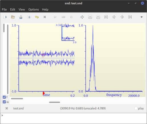
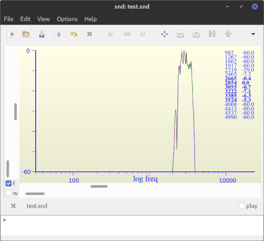
     Above a screenshot of Snd's window showing the timeline waveform on one side and the spectrum (FFT) on the other. Notice the peak around 3000 Hz.

     
     

  2. 
              (with-sound () (bpass-noise 0 2 0.5 1200 500 :len 60))       
     
     
     

     A function call above for “bpass-noise” with a center frequency of 1200 Hz., a bandwidth of 500 Hz., and filter order of 60. Listen and look at the new spectra. Band should be narrower.

     
     

  3. 
              (with-sound () (bpass-noise 0 2 0.5 3000 1000 :len 100))       
     
     
     

     And finally above, a function call with a filter order of 100. Frequency peak of 3000 Hz, should be sharper.

     

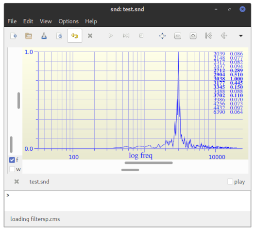
     A screenshot of Snd's spectrum (FFT) window with the filter response. Notice that peaks are very close to 3000 Hz. We might call this a successful implementation of a Bandpass FIR filter.

Next another rendition of a Bandpass but this time using the Butterworth type. Once again there is an example on dsp.scm also adapted and written for Snd by Bill Schottstaedt. More information about Butterworth filters: “HERE”.. A thorough description of “dsp.scm” and its implementation is of course found on Snd's documentation.. Main characteristic of Butterworth filters is having a flat response and though suitable for occasions when a stable pass band is needed. Filter structure definition as well as its implementation on Snd's s7 is provided as follows:

 		 
(define (make-butter-band-pass fq bw)
  (let* ((c (/ 1.0 (tan (* 0.5 (hz->radians bw)))))
	 (d (* 2.0 (cos (hz->radians fq))))
	 (c1 (/ 1.0 (+ 1.0 c)))	)
    (make-filter 3
		 (float-vector c1 0.0 (- c1))
		 (float-vector 0.0
			       (* (- c) d c1)
			       (* (- c 1.0) c1) )) ))


(define butter-band-pass filter)

(define* (butterw start dur amp cfq bw) 
  (let* ((beg (seconds->samples start))
	 (f0 (make-butter-band-pass cfq bw))
	 (ra (make-rand :frequency sampling-rate 
			:amplitude (* 2 amp)))
         (end (+ beg (seconds->samples dur))))
    (do ((i beg (+ i 1)))
	((= i end))
      (outa i (* (* 5 amp) (butter-band-pass f0 (rand ra))))
      )))

Copy-and-paste -all-of-the-above- code into a new file and save it as “butterworth.cms”.

• Load “butterworth.cms”into Snd:

  
           (load "butterworth.cms")        
  
  
  

• Now we can try couple of function calls and listen the effect of a Butterworth on a noise source. On the function definition “butterw” last couple of arguments are center frequency and bandwidth. On the first case we have a center frequency of 1200 Hz. and a very narrow bandwidth of 80 Hz. On the second case we are again trying a a center frequency of 3000 Hz. and a narrow bandwidth of 80 Hz. Take a look at Snd's spectrum screenshot below.

  
  

  1. 
              (with-sound () (butterw 0 2 0.5 1200 80))       
     
     
     

  2. 
              (with-sound () (butterw 0 2 0.5 3000 100))       
     
     
     
     

     A screenshot of Snd's spectrum (FFT) window with the filter response. Notice a filter's flat response and peaks very close to 3000 Hz.

The canonical 'biquad' filter is a second-order IIR filter with two poles and two zeros. In practical terms, it is a versatile filter with options for a wide variety of implementations such as lowpass, highpass, bandpass, notch filter, among others. As an IIR filter, recall that each application depends on the coefficients of its difference equation. Nonetheless, below we are applying coefficients such that we have a resonance filter, almost like a Helmholtz 'resonator', if we can call it like that.

 		 
(define (make-biquad a0 a1 a2 b1 b2)
  (make-filter 3 
	       (float-vector a0 a1 a2) 
	       (float-vector 0.0 b1 b2)))


(define (make-resonance-biquad freq r)                   ;; frequncies in Hz.
  (let* ((radius (- 1. (hz->radians (* r .225))))        ;; radius is bandwidth.
	 (b1 (* -2 radius (cos (hz->radians freq))))
	 (b2 (*  radius radius))
	 (a0 (- 0.5 (* 0.5 b2)))
	 (a1 0.0)
	 (a2 (- a0)))
    (make-biquad a0 a1 a2 b1 b2)) )

(define resonance-biquad filter)


(define* (res-bq start dur freq amp fc ra) 
  (let* ((beg (seconds->samples start))
         (s (make-pulse-train :frequency freq)) 
	 (res (make-resonance-biquad fc ra))
	 (end (+ beg (seconds->samples dur))) )
    (do ((i beg (+ i 1)))
	((= i end))
      (outa i (* 14 amp (resonance-biquad res (pulse-train s))))
      )))

Copy-and-paste this code into a new file and save it as “resonance.cms”.

• Load “resonance.cms”into Snd:

  
           (load "resonance.cms")        
  
  
  

• Coming, two function calls to outline the effect of a Resonance on a pulse train sound source. On the function definition “res-bq” we have arguments for center frequency and bandwidth as well. On the first case we have a center frequency of 3000 Hz. and a bandwidth of 1200 Hz. for natural resonance response. On the second case we are again trying a resonance at 3000 Hz. using a narrower bandwidth of 200 Hz. Listen and take a look at Snd's spectrum screenshot below.

  
  

  1. 
              (with-sound () (res-bq 0 2 1000 0.5 3000 1200))       
     
     
     

  2. 
              (with-sound () (res-bq 0 2 600 0.5 3000 200))       
     
     
     
     

     A screenshot of Snd's spectrum (FFT). Look at the filter's response of this sound and a resonance near 3000 Hz.

Last example is a feedback Comb filter. Comb filters are basic building blocks for digital audio effects. For example acoustic echo simulation is one instance of a comb filter. The feedback comb filter is a special case of an IIR “recursive” digital filter, since there is feedback from the delayed output to the input. The feedback comb filter can be regarded as a series of echoes, exponentially decaying and uniformly spaced in time. There can be time varying comb filters that produce “effects”, such as flanging, phasing and chorusing among others. Snd's comb filter implementation is a delay line with a scaler on the feedback. On this example we are time changing frequencies of the combs so that a changing resonance is heard as time goes by.

 		 
(define* (comb-filter-tv start dur freq amp length feedback
		(chg-env '(0 1 1 0)))                 
  (let* ((beg (seconds->samples start))
	 (end (seconds->samples (+ start dur)))
         (s (make-pulse-train :frequency freq))     ;; pulse train sound source
         (del (make-comb :size length               ;; length of delay (samples)
			:max-size 95
			:scaler feedback))          ;; comb feedback scaler
         (chg (make-env :envelope chg-env           ;; time changing envelope
			  :scaler length
			  :base 10.0
			  :duration dur)))
    (do ((i beg (+ i 1)))
	((= i end))
      (outa i (* amp (comb del (pulse-train s) (env chg))))) ))

Copy-and-paste this code into a new file and save it as “combfilter.cms”.

• Load “combfilter.cms”into Snd:

  
           (load "combfilter.cms")       
  
  
  

• Right below, several function calls showing a comb effect while using a Comb Filter on a pulse train sound source. On the function definition “comb-filter-tv” (i.e. comb filter time variant) we have arguments for delay length, a feedback gain scaler and a time-changing envelope in addition to the other standard parameters. On case first we use a delay of 80 samples and a feedback gain of 0.75. On the second we are using same values but inverting the time envelope. On last couple of examples we tweaking the feedback gain parameter but decreasing delay. Keep on mind that filter gain can over blow since we are feeding back signal.Listen and take a look at Snd's spectrum screenshot below.

  
  

  1. 
              (with-sound () (comb-filter-tv 0 3 600 .3 80 .75))       
     
     
     

  2. 
              (with-sound () (comb-filter-tv 0 3 600 .3 80 .75 :chg-env '(0 0 1 1)))       
     
     
     

  3. 
              (with-sound () (comb-filter-tv 0 3 600 .4 40 .9 :chg-env '(0 0 1 1)))       
     
     
     

  4. 
              (with-sound () (comb-filter-tv 0 3 600 .6 45 .8 :chg-env '(0 0 0.5 .6 1 0)))       
     
     
     
     

     A screenshot of Snd's spectrum (FFT). Look at the filter's response of this sound showing combs at almost middle of the sound file.