Impulse Response

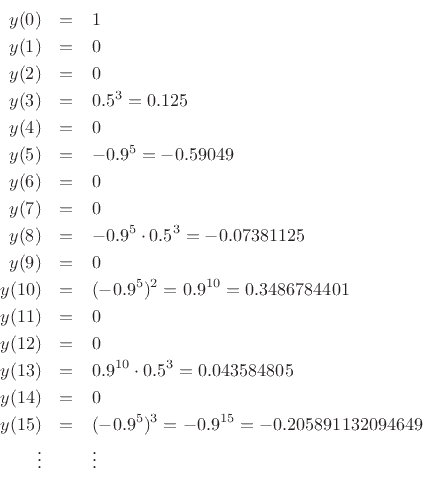
Figure 3.8 plots the impulse response of the example filter, as computed by the matlab script shown in Fig.3.9. (The plot-related commands are also included for completeness.^4.2) The impulse signal consists of a single sample at time 0 having amplitude 1, preceded and followed by zeros (an ideal ``click'' at time 0). Linear, time-invariant filters are fully characterized by their response to this simple signal, as we will show in Chapter 4.

Figure 3.8: Impulse response of the example filter $y(n) = x(n) + 0.5^3 x(n-3) - 0.9^5 y(n-5)$ .

Figure 3.9: Matlab script for computing and plotting the impulse response of the example digital filter.

 

% Example comb filter:
g1 = 0.5^3;  B = [1 0 0 g1];      % Feedforward coeffs
g2 = 0.9^5;  A = [1 0 0 0 0 g2];  % Feedback coefficients

h = filter(B,A,[1,zeros(1,50)]);  % Impulse response
% h = impz(B,A,50); % alternative in octave-forge or MSPTB

% Matlab-compatible plot:
clf; figure(1); stem([0:50],h,'-k'); axis([0 50 -0.8 1.1]);
ylabel('Amplitude'); xlabel('Time (samples)'); grid;
cmd = 'print -deps ../eps/eir.eps'; disp(cmd); eval(cmd);

The impulse response of this filter is also easy to compute by hand. Referring to the difference equation

$$y(n) = x(n) + 0.5^3 x(n-3) - 0.9^5 y(n-5)$$

and setting the input $x(n)$ to $\delta(n) = [1,0,0,\dots]$ , we compute, for $n=0,1,2,\dots$ ,

$$\begin{eqnarray*} y(0) &=& 1\\ y(1) &=& 0\\ y(2) &=& 0\\ y(3) &=& 0.5^3 = 0.125 \\ y(4) &=& 0\\ y(5) &=& -0.9^5 = -0.59049\\ y(6) &=& 0\\ y(7) &=& 0\\ y(8) &=& -0.9^5\cdot 0.5^3 = -0.07381125\\ y(9) &=& 0\\ y(10) &=& (-0.9^5)^2 = 0.9^{10} = 0.3486784401\\ y(11) &=& 0\\ y(12) &=& 0\\ y(13) &=& 0.9^{10}\cdot 0.5^3 = 0.043584805\\ y(14) &=& 0\\ y(15) &=& (-0.9^5)^3 = -0.9^{15} = -0.205891132094649\\ \vdots && \vdots\\ \end{eqnarray*}$$