Next |
Prev |
Up |
Top
|
Index |
JOS Index |
JOS Pubs |
JOS Home |
Search
As noted in [25] et al., it is natural in
practice to implement the junction load impedance (or admittance) as
bank of parallel biquads:
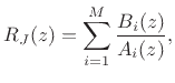 |
(C.102) |
where  is the number of biquads, and we define
A hasty implementation of Eq.(C.97) might overlook
the fact that all junction transfer-functions (transmittances,
reflectances, etc.) must have the same poles (or some subset of
them). It is therefore typical to share the pole computations
among all junction transfer functions, that is, implement the
recursive part only once, and form all desired junction transfer
functions as linear combinations of the same state variables (or
biquad sections, etc.). Thus, only the numerators differ
between the driving-point impedance  and reflectances
 , for example. The ``dynamics'' are shared
because there is only one physical system being modeled, but the inputs
and outputs vary, yielding different zeros.
, for example. The ``dynamics'' are shared
because there is only one physical system being modeled, but the inputs
and outputs vary, yielding different zeros.
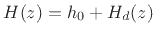
A basic trick for implementing the reciprocal of a transfer
function without altering its denominator(s) is to place it in
a feedback loop. If
 denotes the starting
transfer function, then placing it in a feedback loop gives
denotes the starting
transfer function, then placing it in a feedback loop gives
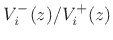
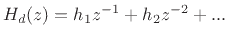
 . Now split
  into its instantaneous and delayed
components
into its instantaneous and delayed
components
 , where
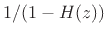
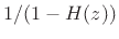
 . If
. If 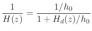 (otherwise pull out unit-sample delays until it is),
then we can realize
(otherwise pull out unit-sample delays until it is),
then we can realize  as
as
 |
(C.105) |
which can be implemented as a feedback loop containing
 as the feedback filter, and the scale factor
  in the forward path, as shown in Fig.C.30.
In the case of a parallel biquad realization, structure is preserved
with altered numerators obtained by extracting the instantaneous gain
from each section, as we'll see the following examples.
in the forward path, as shown in Fig.C.30.
In the case of a parallel biquad realization, structure is preserved
with altered numerators obtained by extracting the instantaneous gain
from each section, as we'll see the following examples.
Figure C.30:
Feedback arrangement for inverting the filter
while preserving
parallel-biquads structure.
![\includegraphics[width=0.6\twidth]{eps/InvertFilter}](img3986.png) |
Subsections
Next |
Prev |
Up |
Top
|
Index |
JOS Index |
JOS Pubs |
JOS Home |
Search
[How to cite this work] [Order a printed hardcopy] [Comment on this page via email]