Next |
Prev |
Up |
Top
|
Index |
JOS Index |
JOS Pubs |
JOS Home |
Search
Generalized Scattering Coefficients
Generalizing the scattering coefficients at a multi-tube intersection
(§C.12) by replacing the usual real tube wave impedance
 by the complex generalized wave impedance
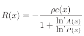
from Eq.(C.173), or, as a special case, the conical-section wave impedance
![$ R_A^\pm (s)=[\rho c/A(x)]/[s/(s \pm 1/t_x)]$](img4422.png) from Eq.(C.172),
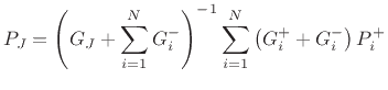
we obtain the junction-pressure phasor [440]
from Eq.(C.172),
we obtain the junction-pressure phasor [440]
where  is the complex, frequency-dependent, incoming,
acoustic admittance of the
is the complex, frequency-dependent, incoming,
acoustic admittance of the  th branch at the junction,
  is
the corresponding outgoing acoustic admittance,
is
the corresponding outgoing acoustic admittance,  is the
incoming traveling pressure-wave phasor in branch
,
is the
incoming traveling pressure-wave phasor in branch
,
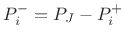 is the outgoing wave, and
  is the admittance of a load at
the junction, such as a coupling to another simulation. For
generality, the formula is given as it appears in the multivariable
case.
is the admittance of a load at
the junction, such as a coupling to another simulation. For
generality, the formula is given as it appears in the multivariable
case.
Next |
Prev |
Up |
Top
|
Index |
JOS Index |
JOS Pubs |
JOS Home |
Search
[How to cite this work] [Order a printed hardcopy] [Comment on this page via email]