Timoshenko's Beam Equations

Timoshenko's theory of beams constitutes an improvement over the Euler-Bernoulli theory, in that it incorporates shear and rotational inertia effects [77]. This is one of the few cases in which a more refined modeling approach allows more tractable numerical simulation; the reason for this is that Timoshenko's theory gives rise to a hyperbolic system, unlike the Euler-Bernoulli system, for which propagation velocity is unbounded. It is this partially parabolic character of the Euler-Bernoulli system which engenders severe restrictions on the maximum allowable time step (at least in the case of explicit methods, of which type are all the scattering-based methods included in this work). For a physical derivation of Timoshenko's system, we refer the reader to [77,146,152,187,188], and simply present it here:

$$\begin{eqnarray}\rho A\frac{\partial^{2}w}{\partial t^{2}} &=& \f... ...\right)+A\kappa G\left(\frac{\partial w}{\partial x}-\psi\right) \end{eqnarray}$$ (5.17a)

As before, $w(x,t)$ represents the transverse displacement of the beam from an equilibrium state, and the new dependent variable $\psi(x,t)$ is the angle of deflection of the cross-section of the beam with respect to the vertical direction. Here, the quantities $\rho$, $A$, $E$ and $I$ are as for the Euler-Bernoulli Equation (5.1). $G$ is the shear modulus (usually called $\mu$ in other contexts) and $\kappa$ is a constant which depends on the geometry of the beam. For generality, we assume that all these material parameters are functions of $x$. Losses or sources are not modeled.

Nitsche [131], in his MDWD network-based approach preferred to use the more fundamental set of four first order PDEs from which system (5.16) is condensed:

$$\begin{eqnarray}\rho A \frac{\partial v}{\partial t} &=& \frac{\p... ...{\partial q}{\partial t} &=& \frac{\partial v}{\partial x}-\omega\end{eqnarray}$$ (5.18a)

$$\begin{eqnarray}\rho I \frac{\partial \omega}{\partial t} &=& \fr... ...ac{\partial m}{\partial t} &=& \frac{\partial \omega}{\partial x}\end{eqnarray}$$ (5.19a)

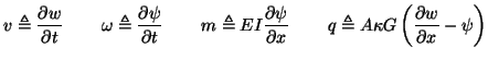
We have introduced here the quantities

$$v\triangleq \frac{\partial w}{\partial t}\hspace{0.3in} \omega\tr... ...ce{0.3in} q \triangleq A\kappa G\left(\frac{\partial w}{\partial x}-\psi\right)$$

$v$ is interpreted as transverse velocity, $\omega$ as an angular velocity, $m$ as the bending moment, and $q$ as the shear force on the cross-section. Each of the subsystems (5.17) and (5.18) has the form of a lossless (1+1)D transmission line system; they are coupled by constant-proportional terms, and it is this coupling that gives the Timoshenko system its dispersive character. The Euler-Bernoulli system (5.4) is recovered in the limit as $A\kappa G\rightarrow\infty$ and $\rho I\rightarrow 0$ [131].

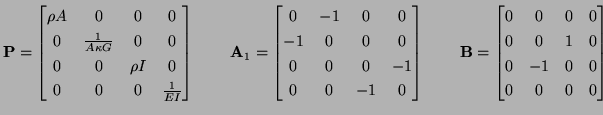
This is a symmetric hyperbolic system of the form given in (3.1), with ${\bf w} = [v, q, \omega, m]^{T}$, ${\bf f} = {\bf0}$ and

$${\bf P} = \begin{bmatrix}\rho A&0&0&0\\ 0&\frac{1}{A\kappa G}&0&0... ...{\bf B} = \begin{bmatrix}0&0&0&0\\ 0&0&1&0\\ 0&-1&0&0\\ 0&0&0&0\\ \end{bmatrix}$$