Speed of Sound and an Open-Ended Tube

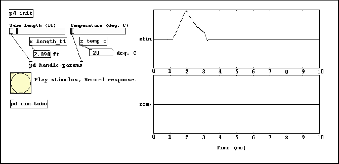
1. Download the pd patch vir_tube1.pd, and open it in pd. Figure 1 shows a sample screen capture of the patch.

2. The patch simulates a single acoustic tube, driven at one end by the stimulus signal shown as stim in the patch, and open at the other end. The applied stimulus results in a right-traveling pressure wave along the tube. The tube length, along with the temperature of the air inside the tube, are adjustable using the sliders shown on the patch. Finally, a sensor located at the stimulus-driven end of the tube measures the left-traveling pressure wave response due to stim, and stores and displays the result at resp.

3. Adjust the temperature to the minimum possible value ($-20^\circ$ C). Next adjust the tube length to approximately 2 ft.

4. If you wish, modify the signal stim using the mouse. Ideally, there should be at least one key visible feature of the stimulus signal aligned with the tick marks on the edges of the plot.

5. To launch the pressure-wave stimulus signal into the tube, click the large circular button. You should see the reflected wave in the resp signal plot.

6. What do you notice about the polarity of the reflected wave?

7. Using the stim and resp graphs, estimate the delay between the stimulus and the response signals. Given the length of the tube, calculate an approximate estimate of speed of sound in the tube. What is the percentage error between this estimate and the theoretical value based on the temperature in the tube?

8. Next adjust the temperature in the tube to a different value using the sliders, and repeat the previous three steps. How does an increase in temperature affect the speed of sound in the tube?

Figure 1: Screen capture showing open-ended acoustic tube patch with variable tube length and air temperature.