
_______________________________________________________________________________________________________________
John Nolting
CCRMA 2007
________________________________________________________________________________________________________________
424 Quarter Project
Modeling the Orban 111b Spring Reverb
The goal of this project is to learn a bit about modeling spring reverbs. The goal of this project is not to model an entire spring reverb unit through circuit analysis, but to take a look at it's response by testing it with audio signals. The unit under test is the Orban 111b spring reverb. Details on how the springs affect audio, and how the springs look in the Orban 111b will be discussed. The tests will be presented and results will be posted.
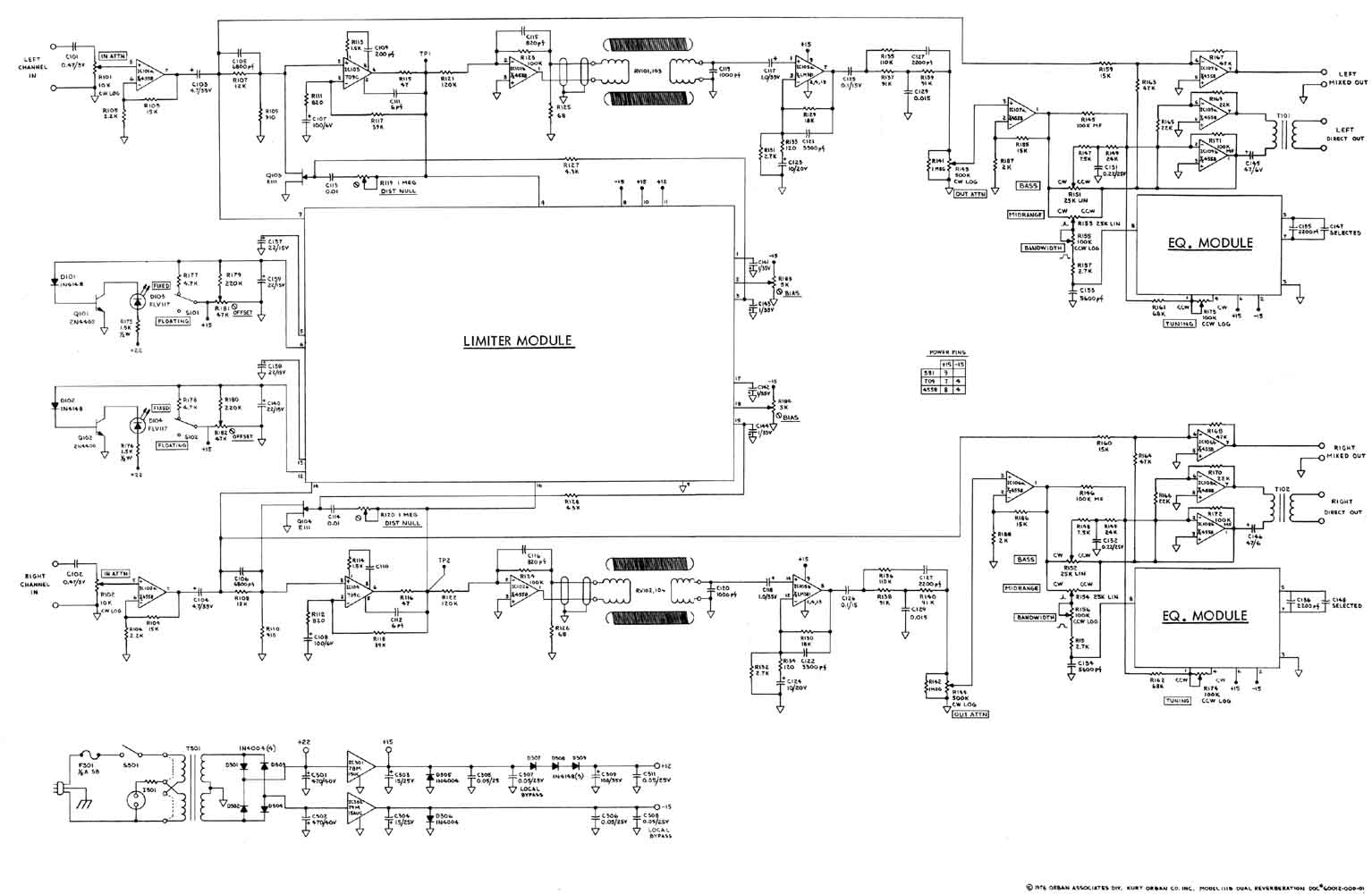
The Orban 111b is a two channel spring reverb.
The schematic for this unit is here .
The manual if here .
The guts, showing the springs, look like this:
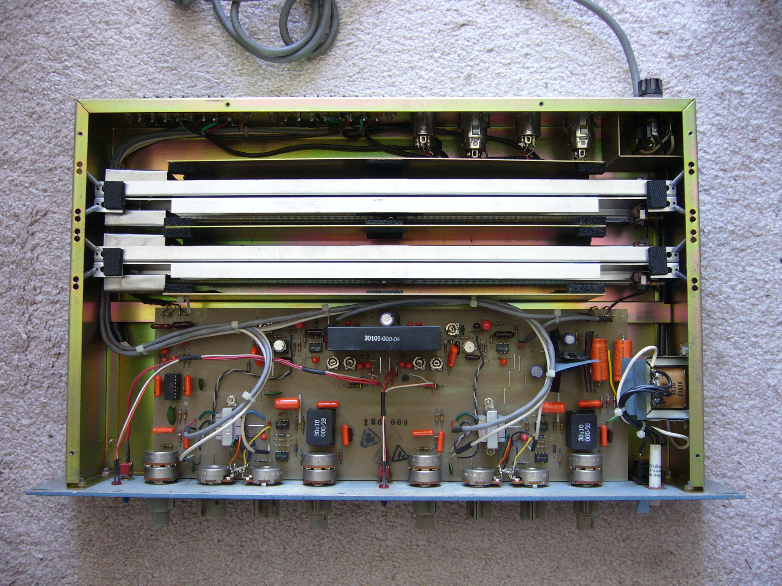
The springs run the full length of the unit (left to right), and are housed within the large metal braces shown above. The metal braces are connected to the units chassis via eight small springs. Audio does not pass through the small springs, they are only used for suspending the housing.
The springs that pass audio are mounted very specific way (described below).
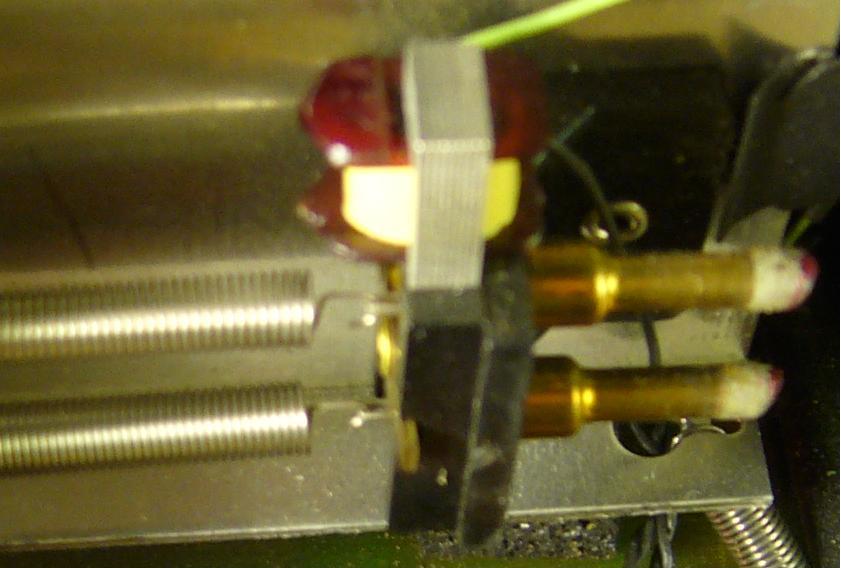
A closer view of one set of the springs looks like this:

Close-up view of one channel of springs
The above picture shows four springs. The springs that are in series are coiled in opposite directions. There are four sets of these series connected springs per channel (making a total of 8 springs per channel, although the manual says 6). The other four springs associated with this channel can't be seen in this photo, but are mounted in a mirrored fashion on the opposite side of the large metal housing.
The springs are affected at one end by a bead that rotates based on the audio input. This rotation induces a torsional wave in the spring, which then moves back and forth along the length of the spring (the direction of a torsional wave is the same as though you were wringing water out of a wet towel, or a twisting direction). The end opposite of the spring is connected to a pick up. The pick up detects the torsional waves in the spring. When a wave reaches the pick up side after being induced by the input side, it is reflected back towards the input. The wave will continue to bounce back and forth between the input and the pick up until the motion is dampened (from reflection loss and heat). So, in the end, the pickup doesn't just see one instance of the input signal, but several instances of the input (each at a later time and lower amplitude).
The torsional waves wind the springs which may create longitudinal waves (the winding of the springs creates spaces between the coils, which result in longitudinal waves along the length of the spring). Longitudinal waves travel at different speeds than torsional waves. In order to minimize longitudinal waves, two springs are connected in series and coiled in opposite directions (this can be seen in the above picture).
This system is similar to a natural room reverb in that with room reverb, a sound will bounce around in a room until it is dampened by reflection loss and air absorption (and several other factors). A listener in a room will hear many instances of the original sound while it is being reflected. This is just like the pick up in a spring reverb, which will 'hear' many instances of the input sound as it is being reflected in the spring.
Now for some testing....
What's the plan?
The general plan here is to run a test signal through the spring reverb and record what happens. The recorded sound and the test sweep are both moved to the frequency domain by taking the FFT of each. Next the FFT of the recorded sound is divided by the FFT of the test sweep. This basically divides out the original test sweep resulting in just the response of the spring reverb. This result is then moved back to the time domain (IFFT), and the real part is taken. This results in the impulse response of the spring reverb. (This can all be done in Matlab.)
The process can be written as: impulse_response = real( IFFT( FFT(recorded_sound) / FFT(test_sweep)))
At this point the impulse response can be used with convolution reverbs to get a reverb sound that sounds exactly like the hardware version of the spring reverb.
The impulses will then be convolved with this input file, just to get an idea of what they sound like on a real signal (drums).
What was done...
Two instances of a sinusoidal log sweep, the second immediately after the first, was passed through the Orban spring reverb.
The test sweep is here .
By 'passed through' I mean the test sweep file was opened in Cubase (a multitrack audio software), played into the Orban spring reverb via a Layla24 sound card, and the output of the Orban spring reverb was recorded back into Cubase on a different track (also via the Layla24 sound card). This process allows for the input and output to have exactly the same start point, and also allows the user to immediately hear the difference between the original test sweep and the test sweep affected by the spring reverb.
The first test was run with the reverb bandwidth set to maximum, all eq's set to zero, and all of the springs undamped.
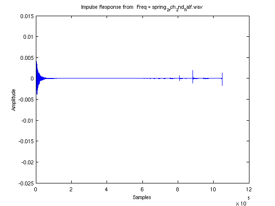
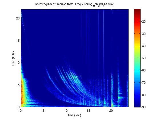
The resulting impulse response and spectrogram are below.

Impulse Response of All of the Springs
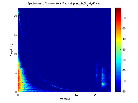
Spectrogram of All of the Springs
This is what this impulse sounded like on a drum kit.
Next, three of the four springs were dampened with foam, and the sweep tests were run again. The idea here is that each spring affects the input signal independently of the other springs. This means that an impulse of each spring can be taken separately, and then an input can be passed through each of the springs separately. The output of the four springs can then be summed (i.e., the springs are summed in parallel).
Dampening the springs with foam looks like this:
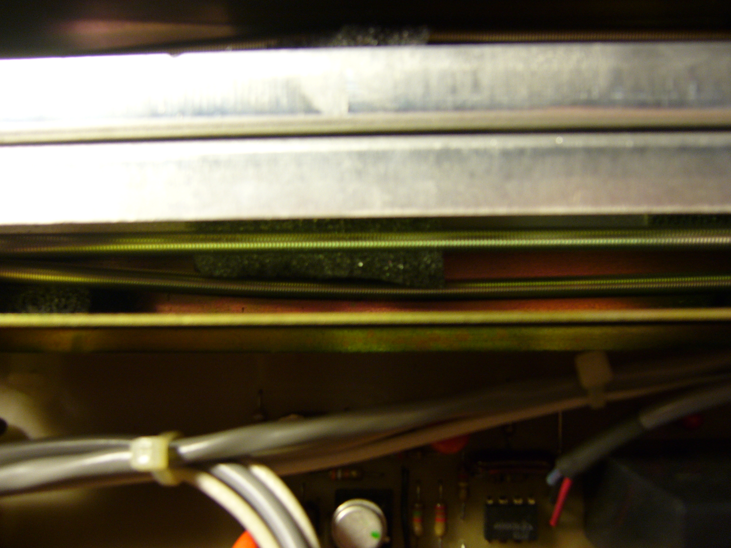
Bottom Spring is Dampened with Foam, Top Spring unaffected
It's a little hard to see in this picture, but both springs on the opposite side of the large metal housing are dampened.
The impulse response of each spring and a Spectrogram of each impulse response is shown below:

Impulse Response of Spring 1
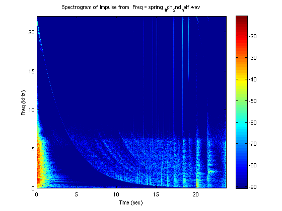
Spectrogram of Spring 1
Impulse Response of Spring 2

Spectrogram of Spring 2

Impulse Response of Spring 3

Spectrogram of Spring 3

Impulse Response of Spring 4
Spectrogram of Spring 4
The drum sample convolved with Spring 1 on its own sounds like this .
Some experimentation was done by taking the recorded impulse sweep of all of the springs combined, and passing it through the Orban spring reverb a second time. This resulted in what would be equivalent to have two spring reverb units in series.
The experimental impulse response when convolved with the drum sample sounds like this .
The generated impulse responses can now be used with a convolution reverb VST plug-in such as SIR . This program allows the user to import their own impulse responses and convolve them with their own samples.
and finally, the generated impulses for the above example are available here:
So, although I liked the sound of the above impulse response, it is not as clean as what is needed to really get a good look at what the spring is doing on its own. There are several impulses appearing after the first impulse. These impulses are the result of some type of non-linearity in the system. This non-linearity can be occurring at any point in the recording process, or can be occurring somewhere in the spring reverb.
First, the foam was repositioned and more tests were taken. The results of these tests did not show any improvement. It is possible that the spring is banging against the metal housing, or vibrating against the foam in some weird way. To insure this is not the case, all of the springs in the channel under test are removed, accept for one (in this case, this spring is being called "spring 2").
Removing the springs for test is NOT recommended. It is very difficult to reconnect them.
The hook connecting the spring to the pickup transducer looks like this:
Spring Connection, One Side Only
After disconnecting the springs, it was found that the springs are different lengths. In retrospect, this should have been assumed, but it never crossed my mind. The different length springs result in different echo times (longer spring, longer time between echoes).
The disconnected springs look like this: (click photo to download hi res image)

Bottom and Top Springs
The two bottom springs add to a total of about 8 inches long, and the top springs are about 10 inches long. This finding is another reason to look at one isolated spring, as opposed to all the springs at one time.
With only one spring connected, the system is ready to test. It is now certain that the other damped springs will not cause any non-linearity while testing.
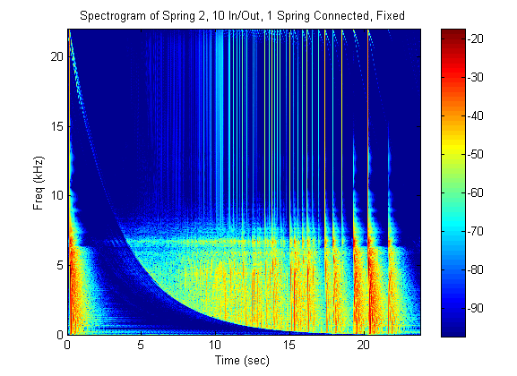
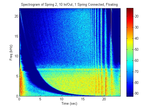
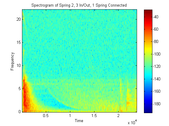
Several trials over a couple of weeks were taken to see what happens at different settings of the spring reverb. There is a switch called fixed/float that is briefly described in the manual. The effect of this switch is not certain, but tests were done at both settings to check the result. It was assumed that this switch affected the limiting circuit, so both high amplitudes and low amplitudes were tested. The reason for this test is to continue the search for the cause of the non-linearity's in the spectrograms.
Two results, when the input and output gain settings were both set to 5 (middle setting), are shown below:


Although the spectrogram in the floating position looks cleaner, neither setting eliminated the non-linearities.
The input and output gains are raised to 10, and the system is tested again:
Obviously, this did not help.
After several tests at different input and output amplitudes, the impulse response with the least non-linearities was chosen. In the interest of time, some analysis will be done to this response.
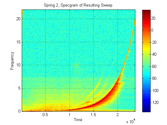
The spectrogram of the impulse chosen for analysis looks like this:
The log sweep, before the impulse response was generated looks like this:
The following plots show the results of a series of tests. The tests include filtering the response into several different bands and analyzing each of these frequency bands separately. The information of interest is T60 (the time it take the frequency band to decay to -60 dB), and the signal to noise ratio of each band.
The following graphs display the the impulse response of six different frequency bands. The frequency bands and SNR values of each of the graphs is displayed above the plot.
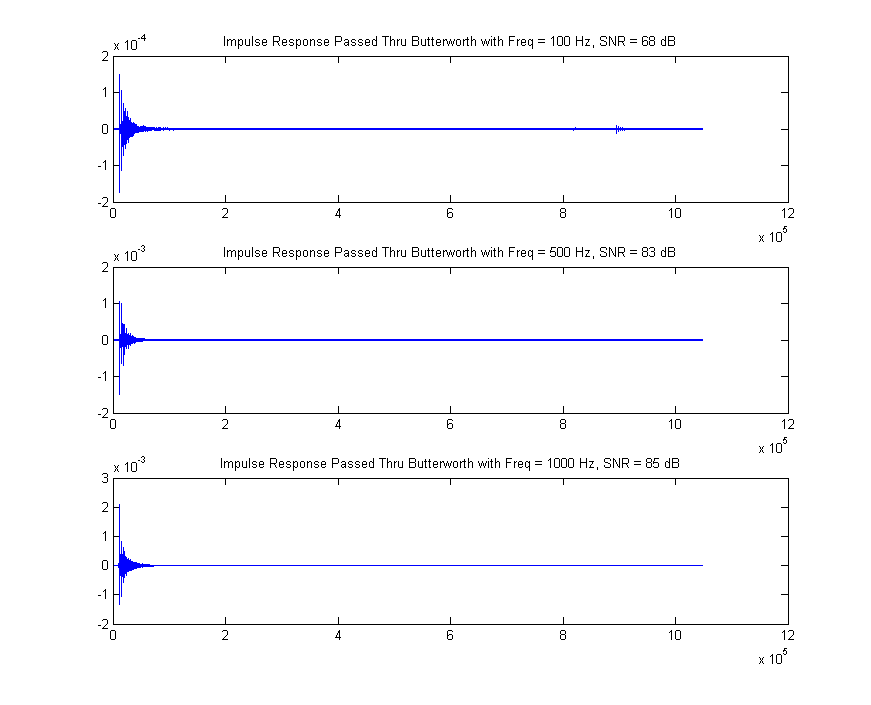

The response has a low SNR at low frequencies. SNR increases until around 1 KHz, and then slowly decreases until 6 KHz.
The following plots show the T60's associated with each of these frequency bands...


The T60 is at about 2 seconds at 100 Hz. The T60 slowly shortens until it reaches about 1.25 seconds at 6 KHz. Further tests were taken that resulted T60's similar to that at 6 KHz all the way to 10KHz. This means that the energy in the lower frequencies is present in the output signal for a longer period of time. In other words, bass sounds have a longer reverb time applied to them than mid and hi sounds.
Finally, the delay in the high frequencies can be seen by looking in close the the impulse response...

This plot shows that the propagation time, or the time it takes for the frequency to move back and forth along the spring, is faster at low frequencies. There is a cutoff at about 6 KHz. Above this cutoff, there is a set of high frequency impulses that appear at a much higher rate than below the cutoff. The high frequency impulses appear to be occurring at about 3 times the rate of the lower frequency impulses.
Matlab scripts created for testing and generating impulses are here:
SNR and Band-limited Impulse Plots
Future work:
It is clear from the above analysis that the generated impulse still has too many non-linearities. To better test the limiter circuit in the system, a sinusoid at a hi amplitude can be added to the test sweep at a low amplitude. This will cause the limiter to detect the amplitude of the sinusoid and not the amplitude of the sweep. The sinusoid can later be extracted and a sweep that is unaffected by the limiter may result. Also, the spring housing can be desoldered and tested outside of the reverb unit. This destructive type of testing is beyond the scope of this project.