 Analysis
General Block Diagram

The tracker algorithm implements high-resolution sinusoidal analysis suitable for both harmonic and non-harmonic sounds. The technique used for tracking partials is similar to the deterministic analysis of Xavier Serra's SMS (Spectral Modeling Synthesis). One difference with SMS's deterministic analysis is that tracker uses also psychoacoustic information to determine the salience of detected peaks. This information (measured as signal-to-mask ratio, or SMR) is derived from masking effects produced within critical bands, and accounts for the audibility of sinusoidal trajectories. To achieve coherent sinusoidal trajectories, both SMR and frequency deviation information are used to track partials across frames .
Tracker consists of five main modules. The windowing module breaks the analyzed sound into sort-time overlapping segments and applies an analysis window to the signal. Windows from the Blackman-Harris family are normally used but any other window type implemented by CLM can be used (see the documentation section below). The hop size (number of samples to skip by the analysis window) is expressed as a proportion of the window size (0.25 means 1/4 of the window). The size of the analysis window is calculated as a function of the number of cycles of the lowest frequency to be tracked by the system (usually the fundamental in the case of harmonic sounds). The size of the Fast Fourier Transform (FFT), used to compute the Short Time Fourier Transform (STFT) in the analysis, is internally calculated as the closest power of two greater than two windows, assuring enough zero padding. Both the window size (M) and the FFT size (N) can be forced to be any number of samples (the condition: M<=N has to be achieved, and N must be a power of 2).
Peak Detection

The spectrum issued from the Short Time Fourier Transform (STFT) of the windowed signal is converted to polar form to obtain the magnitude and phase of each bin. After this, peaks are detected along the dB magnitude spectrum. A peak is a local maximum in the spectrum defined as: |Xk-1| < |Xk| > |Xk+1| where Xk is the peak location and Xk-1, Xk+1 its surrounding bins. Once a peak is detected, its real amplitude, frequency, and phase values are obtained by means of parabolic interpolation. Only peaks with magnitude above an indicated threshold are kept in the analysis. For more details on these peak detection and interpolation techniques you can visit Julius Smith's web page on PARSHL.
Peak Tracking

Peaks detected in one analysis frame have to be integrated to sinusoidal trajectories. This is done in three steps: first, candidates to continue a particular trajectory are found in the peak pool of the new frame; second, the best candidate is found based on masking and frequency information. Trajectory's frequency and SMR are averaged across frames and these values, called tracks, are used to evaluate which peak of the pool better continues the trajectory. An adjustable number of frames is used to average track values, the latest peak incorporated to the trajectory can also be used (in a weighted fashion) to compute track parameters (this can be useful for tracking unstable sinusoids, see the documentation below). The best peak candidate will be the one with minimal SMR difference and frequency deviation from the track (the intervention of masking information in this process can be also weighted, see the documentation below). Taking two parameters into account, SMR and frequency deviation, practically eliminates conflicts between tracks (i.e. having more than one track claiming for the same peak). Finally, tracked peaks are incorporated to their sinusoidal trajectories, trajectories that didn't incorporate peaks in this frame are "turned off" (tracks keep their last values and wait for candidate peaks in subsequent frames), and peaks left over in the pool "start up" new trajectories and tracks.
Psychoacoustic Processing

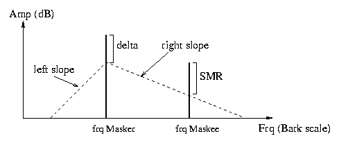
Signal to Mask Ratio (SMR) information used during tracking is computed by the Psychoacoustic Processing module. The magnitude of the peaks present in a frame are used to evaluate a masking threshold across frequency. All peak frequencies are converted to Bark scale and linear masking curves traced up and down in frequency from each peak location (note the asymmetry between the left and right slope of the lines on the picture, the right slope is inversely proportional to the magnitude of the peak). After masking curves for all peaks are traced, they are combined to create a masking threshold across the 25 critical bands (from 1 to 25 Barks). Then SMR for each peak is computed as the ratio in dB between the peak's magnitude and the level of the masking threshold at the peak's location.
Post-processing
After partials were tracked, an ATS-SOUND structure is created to store the spectral data. In a post-processing stage, short trajectories with low SMR average value are removed and gaps in continuous trajectories fixed. Also in this step, frequency centroid and average SMR for each partial are computed and stored in the structure.
Residual

Once sinusoidal trajectories are fixed and stored, the residual is computed. This step is performed by re-synthesizing the tracked partials using phase information, and subtracting them from the original sound in the time domain. The resulting signal is called residual and contains what was left out by the tracking process, usually noise. A two-channel file with the re-synthesis and the residual is generated by the system, and can be used as an intuitive measure of the sinusoidal tracking quality. Normally, a noisy and low-energy residual is sign of successful tracking (see the documentation below).
Residual Analysis

After being computed, the residual is analyzed at frame rate using a sliding rectangular window and the STFT. The fequency spectrum of the residual is transformed to Bark scale and energy computed at each of the 25 critical bands. The residual's energy is then re-injected as modulated narrow-bandwidth noise to partials present at each sub-band of the spectrum. Band regions with significant energy where no partials were tracked are kept in a complementary model. Modulated critical-bandwidth noise is used to model residual energy in those remaining sub-bands regions.
Tracker Documentation
tracker file snd &key (start 0.0)(duration nil)(lowest-frequency 20)(highest-frequency 20000.0)(frequency-deviation 0.1)(window-cycles 4)(force-M NIL)(window-type 'blackman-harris-4-1)(force-window NIL)(hop-size 1/4)(fft-size nil)(lowest-magnitude (db-amp -60))(track-length 3)(last-peak-contribution 0.0)(SMR-continuity 1.0)(amp-threshold nil)(min-segment-length 3)(residual "ats-residual.snd")(verbose nil)
- file: string with the name and path of the soundfile to analyze. Should be a mono file (in case a multichannel file is passed, tracker will automatically analyze its first channel). All soundfile types supported by CLM can be read.
- snd: name of the sound structure to be used in ATS to store the analysis data. This is a Lisp symbol that will point to the ATS-SOUND structure generated by tracker.
- start: time offset in the file where to start the analysis, defaults to 0.0 seconds.
- duration: duration of the analysis in seconds. Defaults to NIL, what means that analysis will be perform until the end of the soundfile is reached.
- lowest-frequency: lowest frequency to track. Peak detection will be performed from this frequency up. This value is also used to compute the size of the analysis window (see window-cycles below), it defaults to 20 Hz.
- highest-frequency: highest frequency to track: peak detection will be performed up to this frequency value. Defaults to 20KHz.
- frequency-deviation: maximum deviation allowed around the frequency of a track. This value is expressed as a proportion of the track's frequency. For instance, a value of 0.1 means that only peaks with frequency values within 10% off a particular track's frequency will be considered candidates for continuation. The smaller this value the more stable trajectories will be tracked, it defaults to 0.1 (10% of the frequency of the track). Note that this parameter works in cojunction with SMR-continuity (see below)
- window-cycles: number of cycles of the lowest-frequency to be present in one analysis window. Defaults to 4 cycles. The analysis window size (M) is computed as:
M = Fs*window-cycles/lowest-frequency [samples] (Fs: sampling rate read from the header of the analysis file). - force-M: this parameter overrides window-cycles, it should be only used in case a particual number of samples is wanted for the window size. Defaults to NIL.
- window-type: analysis window type. ATS has built-in Balckman-Harris windows of 6 types:
- exact-blackman
- blackman
- blackman-harris-3-1
- blackman-harris-3-2
- blackman-harris-4-1
- blackman-harris-4-2
Each type presents a different compromise between main-lobe width and side-lobe rejection. Type blackman-harris-4-1 (-92 dB side-lobe rejection) is used by default. - force-window: this parameter overrides window-type, any type of window implemented by CLM can be used here. Defaults to NIL (i.e. window-type is used).
- hop-size: proportion of the analysis window length (M) to be advanced in time. Default value is 1/4. The analysis frame period in seconds can be computed as:
M*hop-size/Fs - fft-size: forces the FFT size. Defaults to NIL, what means that the FFT size (N) will be calculated as the first power of 2 greater than twice the window size (zero-padding is applied). This parameter should be used only when a particular combination of M and N is wanted (see also force-M).
- lowest-magnitude: lowest magnitude of a peak to be detected, only bins with magnitudes above this value will be considered by the peak detection algorithm. Defaults -60 dB (0.001)
- track-length: length of the analysis tracks in frames. This value affects the "memory" of the peak tracking algorithm (i.e. its ability to predict what a stable trajectory is). For stable sounds you can increase this value (it defaults to 3 frames), for unstable sounds you can make it smaller (with a value of 1 it will track peaks on a frame by frame basis). The parameter last-peak-contribution also affects the way peaks are tracked (see below).
- last-peak-contribution: this parameter controls the weight the last peak incorporated to a trajectory has in the peak tracking process. With the default value 0.0 peak tracking is totally determined by averaged frequency and SMR values called tracks (see track-length above). With a value of 1.0 tracking decisions are made using the last-peak incorporated to a trajectory (tracks are not used). Values in between can be used to account for both stability and sudden trajectory changes.
- SMR-continuity: this parameter controls the weight Signal to Mask Ratio (SMR) information has in the peak tracking process. With the default value 1.0 SMR has equal weight as frequency deviation information, with a value of 0.0 only frequency information is used for tracking peaks. Values in between adjust the amount of SMR continuation wanted in the analysis.
- amp-threshold: this parameter is used during ATS-SOUND post-processing. Only trajectories with an average amplitude over the amp-threshold are kept as sound partials. The default value is NIL, what means that all trajectories will be kept.
- min-segment-length: this parameter is used during ATS-SOUND post-processing. Segments shorter than min-segment-length frames are removed from the trajectories. This helps to avoid keeping intermittent short segments in a sound.
- residual: name of the residual file ATS will generate after analysis. This is a two-channel file, the first channel contains the time-domain residual of the analysis, and the second one the re-synthesis of it (with phase). The default soundfile name is "ats-residual.snd", and will be written in the current directory, a string with a more convenient soundfile name an a path can be used. If NIL is passed, then no residual analysis is performed.
- verbose: print tracking information during analysis. Defaults to NIL.
Examples
;;; clarinet analysis
(tracker (concatenate 'string *ats-snd-dir* "clarinet.aif")
	 'cl
	 :start 0.0
	 :hop-size 1/4
	 :lowest-frequency 100.0
	 :highest-frequency 20000.0
	 :frequency-deviation 0.05
	 :lowest-magnitude (db-amp -70)
	 :SMR-continuity 0.7
	 :track-length 6
	 :min-segment-length 3
	 :residual "/tmp/cl-res.snd"
	 :verbose nil)

;;; crotale analysis
(tracker (concatenate 'string *ats-snd-dir* "crt-cs6.snd")
	 'crt-cs6
	 :start 0.1
	 :lowest-frequency 500.0
	 :highest-frequency 20000.0
	 :frequency-deviation 0.15
	 :window-cycles 4
	 :window-type 'blackman-harris-4-1
	 :hop-size 1/8
	 :lowest-magnitude (db-amp -90)
	 :amp-threshold -80
	 :track-length 6
	 :min-segment-length 3
	 :last-peak-contribution 0.5
	 :SMR-continuity 0.3
	 :residual "/tmp/crt-cs6-res.snd"
	 :verbose nil)


