Let ![]() denote the transverse displacement, in one plane, of a
vibrating string [60]. The complete linear time-invariant
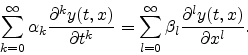
generalization of the lossy, stiff string is described by the differential
equation
denote the transverse displacement, in one plane, of a
vibrating string [60]. The complete linear time-invariant
generalization of the lossy, stiff string is described by the differential
equation
 |
(21) |
 , and sampling
according to
, and sampling
according to
 and
and
 , with
 , (the spatial sampling period is taken to
be frequency invariant, while the temporal sampling interval is modulated
versus frequency using allpass filters), the left- and right-going sampled
eigensolutions become
, (the spatial sampling period is taken to
be frequency invariant, while the temporal sampling interval is modulated
versus frequency using allpass filters), the left- and right-going sampled
eigensolutions become
| (22) |
 . Thus, a general map of
 In summary, a large class of wave equations with constant coefficients, of any order, admits a decaying, dispersive, traveling-wave type solution. Even-order time derivatives give rise to frequency-dependent dispersion and odd-order time derivatives correspond to frequency-dependent losses. Higher order spatial derivatives can be approximated by higher order time derivatives and treated similarly [10]. The corresponding digital simulation of an arbitrarily long (undriven and unobserved) section of 1D medium (such as a string or acoustic tube) can be simplified via commutativity to at most two pure delays and at most two linear, time-invariant filters. In higher dimensions, such as for the 2D mesh, the per-sample filtering cannot in general be exactly commuted to the boundaries of the mesh. However, an approximation problem can be solved which matches the observed modal frequencies and decay rates using sparsely distributed low-order filters in an otherwise lossless mesh (e.g., around the rim).
In practical physical simulation scenarios, such as for real-world strings or acoustic tubes, it is generally most effective to identify experimentally the attenuation and dispersion associated with wave propagation at each frequency over the band of interest [108,49]. These data can be used to design a digital filter which gives an optimal approximation over the propagation distance desired. If needed, the per-sample filter identified in this way can be translated into higher-order terms in the wave equation for the medium. Thus, the wave equation itself can be ``identified'' from measured input-output behavior of the medium (assuming it is linear and uniform) rather than being derived from physical principles and physical constants of the medium as is classically done [61,11].