The Cubic Rectilinear Scheme

This is the simplest scheme for the (3+1)D wave equation. The grid points, indexed by $i$, $j$ and $k$ are located at coordinates 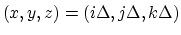$(x,y,z) = (i\Delta, j\Delta, k\Delta)$. The finite difference scheme is written as

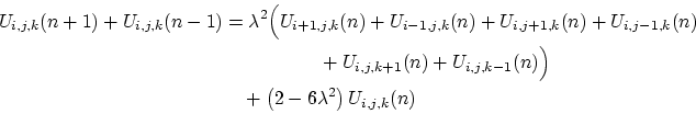$$\begin{split}U_{i,j,k}(n+1)+U_{i,j,k}(n-1) &= \lambda^{2}\Big... ...)\\ &\quad +\left(2-6\lambda^{2}\right)U_{i,j,k}(n) \end{split}$$ (27)

If the grid points are located at the corners of a cubic lattice, then updating the scheme requires access to the grid function at the six neighboring corners; see Figure 8(a). The stability analysis is very similar to that of the (2+1)D rectilinear scheme, except that we now have a 3-tuple of spatial frequencies, $\beta$$= [\beta_{x}, \beta_{y}, \beta_{z}]^{T}$. The amplification polynomial equation is again of the form of (5), with

$$B_{\mbox{{\scriptsize\boldmath$\beta$}}} = -2\left(1+\lambda^{2}\... ...os(\beta_{x}\Delta)+\cos(\beta_{y}\Delta)+\cos(\beta_{x}\Delta)-3\right)\right)$$

and thus

$$F_{\mbox{{\scriptsize\boldmath$\beta$}}} = \cos(\beta_{x}\Delta)+\cos(\beta_{y}\Delta)+\cos(\beta_{x}\Delta)-3$$

Because $F_{\mbox{{\scriptsize\boldmath $\beta$}}}$ is multilinear in the cosines, it is simple to show that

$$\max_{\mbox{{\scriptsize\boldmath$\beta$}}}F_{\mbox{{\scriptsize\... ...ox{{\scriptsize\boldmath$\beta$}}}F_{\mbox{{\scriptsize\boldmath$\beta$}}} = -6$$

and so, from (9),

$$\lambda\leq\frac{1}{\!\!\sqrt{3}}$$

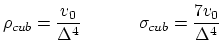
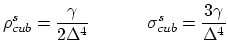
When $\lambda = 1/\sqrt{3}$, the amplification factors become degenerate and linear growth of the solution may occur for $\beta_{x} = \beta_{y} = \beta_{z} = 0$, and for $\vert\beta_{x}\vert=\vert\beta_{y}\vert=\vert\beta_{z}\vert = \pi/\Delta$. The computational and add densities are

$$\rho_{cub} = \frac{v_{0}}{\Delta^{4}}\hspace{0.5in}\sigma_{cub} = \frac{7v_{0}}{\Delta^{4}}$$

for $v_{0}>\sqrt{3}\gamma$, and

$$\rho^{s}_{cub} = \frac{\gamma}{2\Delta^{4}}\hspace{0.5in}\sigma^{s}_{cub} = \frac{3\gamma}{\Delta^{4}}$$

at the stability limit $v_{0} = \sqrt{3}\gamma$. At this limit, the scheme may, like the (2+1)D scheme, be divided into two mutually exclusive subschemes. See Figure 8(b) and (c) for plots of the numerical dispersion properties of the cubic rectilinear scheme.