Practical Bottom Line

Since we must use the DFT in practice, preferring an FFT for speed, we typically compute the sample autocorrelation function for a length $M$ sequence $v(n)$ , $n=0,1,2,\ldots,M-1$ as follows:

1. Choose the FFT size $N$ to be a power of 2 providing at least $M-1$ samples of zero padding ( $N\geq 2M-1$ ):

   $$x \isdef [v(0),v(1),\ldots,v(M-1), \underbrace{0,\ldots,0}_{\hbox{$N-M$}}].$$ (7.21)

   
   

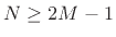
2. Perform a length $N$ FFT to get $X(\omega_k)=\hbox{\sc FFT}_k(x)$ .
3. Compute the squared magnitude $\left\vert X(\omega_k)\right\vert^2$ .
4. Compute the inverse FFT to get $(x\star x)(l)$ , $l=0,\ldots,N-1$ .
5. Remove the bias, if desired, by inverting the implicit Bartlett-window weighting to get

   $$\hat{r}_{v,M}(l) \isdef \left\{\begin{array}{ll} \frac{1}{M-\vert l\vert} (x\star x)(l), & l=0,\pm1,\pm2,\pm M-1\;\mbox{(mod $N$)} \\ [5pt] 0, & \vert l\vert\geq M\; \mbox{(mod $N$)}. \\ \end{array} \right.$$ (7.22)

   
   

Often the sample mean (average value) of the $M$ samples of $v(n)$ is removed prior to taking an FFT. Some implementations also detrend the data, which means removing any linear ``tilt'' in the data.^7.6

It is important to note that the sample autocorrelation is itself a stochastic process. To stably estimate a true autocorrelation function, or its Fourier transform the power spectral density, many sample autocorrelations (or squared-magnitude FFTs) must be averaged together, as discussed in §6.12 below.