Next |
Prev |
Up |
Top
|
Index |
JOS Index |
JOS Pubs |
JOS Home |
Search
Equations of motion for any physical system
may be conveniently
formulated in terms of the state of the system [333]:
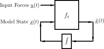
![$\displaystyle \underline{{\dot x}}(t) = f_t[\underline{x}(t),\underline{u}(t)] \protect$](img204.png) |
(2.6) |
Here,
 denotes the state
of the system at time
denotes the state
of the system at time  ,
,
 is a vector of external
inputs (typically forces), and the general vector function
is a vector of external
inputs (typically forces), and the general vector function  specifies how the current state
and inputs
cause a
change in the state at time
by affecting its time derivative
specifies how the current state
and inputs
cause a
change in the state at time
by affecting its time derivative
 . Note that the function
may itself be time varying
in general. The model of Eq.(1.6) is extremely general for
causal physical systems. Even the functionality of the human brain is
well cast in such a form.
. Note that the function
may itself be time varying
in general. The model of Eq.(1.6) is extremely general for
causal physical systems. Even the functionality of the human brain is
well cast in such a form.
Equation (1.6) is diagrammed in Fig.1.4.
The key property of the state vector
in this formulation is
that it completely determines the system at time
, so that
future states depend only on the current state and on any inputs at
time
and beyond.2.8 In particular, all past states and the
entire input history are ``summarized'' by the current state
.
Thus,
must include all ``memory'' of the system.
Subsections
Next |
Prev |
Up |
Top
|
Index |
JOS Index |
JOS Pubs |
JOS Home |
Search
[How to cite this work] [Order a printed hardcopy] [Comment on this page via email]