 |
Figure 2.15 shows the general case of an input signal that interacts with the state of the system at one point along the waveguide. Since the interaction is physical, it only depends on the ``incoming state'' (traveling-wave components) and the driving input signal.
| |
A less general but commonly encountered case is shown in Fig.2.16. This case requires the ``outgoing disturbance'' to be distributed equally to the left and right, and it sums with the incoming waves to produce the outgoing waves.
Figure 2.17 shows a further reduction in generality--also commonly encountered--in which the interaction depends only on the amplitude of the simulated physical variable (such as string velocity or displacement). The incoming amplitude is formed as the sum of the incoming traveling-wave components. We will encounter examples of this nature in later chapters (such as Chapter 9). It provides realistic models of physical excitations such as a guitar plectra, violin bows, and woodwind reeds.
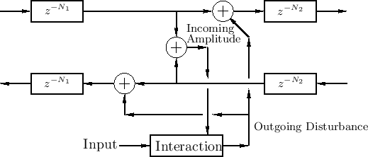 |
If an output signal is desired at this precise point, it can be computed as the incoming amplitude plus twice the outgoing disturbance signal (equivalent to summing the inputs of the two outgoing delay lines).
Note that the above examples all involve waveguide excitation at a single spatial point. While this can give a sufficiently good approximation to physical reality in many applications, one should also consider excitations that are spread out over multiple spatial samples (even just two).
We will develop the topic of digital waveguide modeling more systematically in Chapter 6 and Appendix C, among other places in this book. This section is intended only as a high-level preview and overview. For the next several chapters, we will restrict attention to normal signal processing structures in which signals may have physical units (such as acoustic pressure), and delay lines hold sampled acoustic waves propagating in one direction, but successive processing blocks do not ``load each other down'' or connect ``bidirectionally'' (as every truly physical interaction must, by Newton's third law3.6). Thus, when one processing block feeds a signal to a next block, an ``ideal output'' drives an ``ideal input''. This is typical in digital signal processing: Loading effects and return waves3.7 are neglected.3.8
