Simulation Results

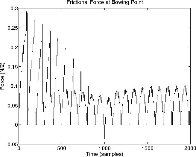
Figure 3 displays waveforms generated by the bow-string model given a constant bow force, velocity, and position. The frictional force applied to the string by the bow can be seen to diminish as the oscillation develops. The string displacement near the bridge clearly exhibits the single main impulse once per period associated with canonical Helmholtz bowed-string motion; there are also many secondary impulses associated with the ringing of the piece of the string between the bridge and the bow. The complexity control will determine whether these secondary impulses are included or suppressed.

Figure: Output of the bow-string model before extracting bridge impulses. Top: Frictional force between bow and string. Middle: String displacement $1/2$ sample from the bridge. Bottom: Sound pressure radiated from simulated body filter. Bowing parameters (fixed): speed 15 cm/sec, force 20 grams, position 3 cm from bridge. A two-pole, two-zero bridge-filter for a digital waveguide string model was calibrated to measurements of violin pizzicato waveforms. A torsional-wave loss coefficient of 0.9 was implemented at the bow at all times.

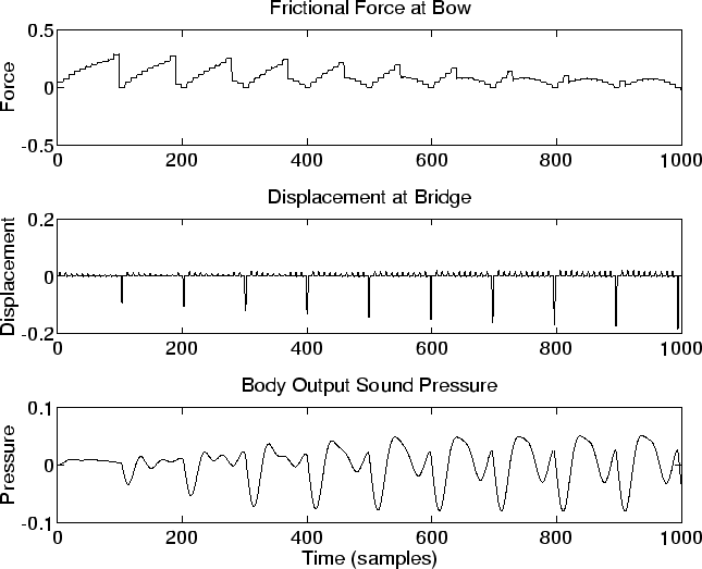Figure 4 illustrates the samples of bridge displacement waveform over a longer period of time. Note that each main Helmholtz impulse plots as two adjacent samples, indicating that a single-sample impulse is traveling on the string. (The observation point is 1/2 spatial sample from the bridge, so that a single impulse at the bridge appears twice, both before and after reflection at the bridge.) Note also that late in the stroke, a strong secondary impulse has developed, making the sound tend toward an octave higher. This ``sul ponticello'' sound is associated with insufficient bow force.

Figure: String displacement $1/2$ sample from the bridge over four short time intervals spanning 1.7 seconds.

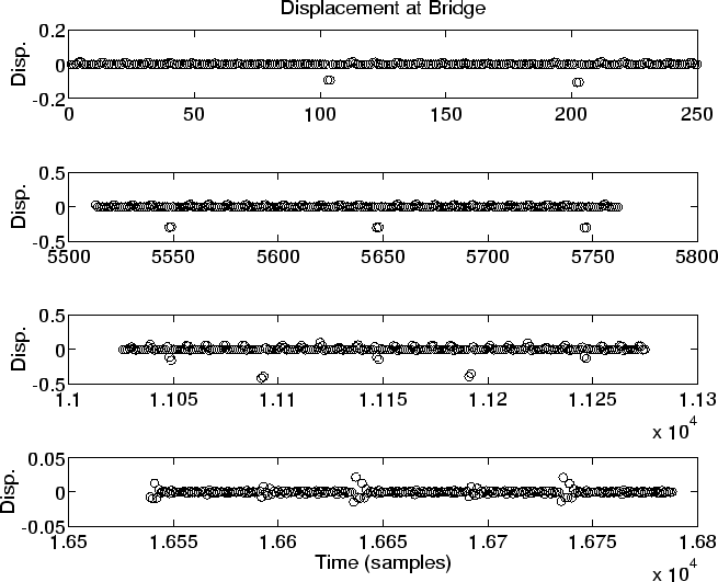Figure 5 gives a close-up of the frictional force during the initial attack transient. As can be seen, even though the applied bow force and velocity are constant, a highly complex interaction occurs between the bow and string.

Figure: Close up of the frictional force waveform during the initial attack.

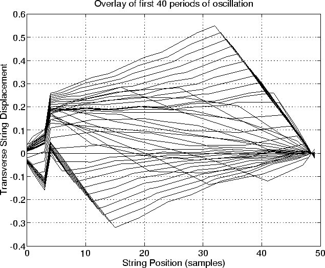
Figure 6 shows an overlay of the first 40 periods of oscillation of the bowed string, with each string snapshot taken slightly later than one period after the previous, and the first snapshot being taken at time zero. The bow is at the sharp upper corner on the left. Note that the vertical scale is highly magnified relative to the horizontal scale. There is also some distortion in the string shape resulting from the lumping of the string losses at the bridge and bowing point, as is typical in waveguide string modeling.

Figure: Snapshots of string state for first 40 periods of oscillation.